
AI-410 · Lesson 2 of 12 · 27 min
Attention, positions and long context
Lesson 1 described a large language model as a stack of transformer blocks trained to predict the next token. This lesson looks inside the part of the block that gives transformers their power and most of their cost: attention. We review how causal self-attention works in a language model, how models know where each token sits in the sequence, why the memory needed to generate text grows with the length of the context, and the techniques that have stretched context windows from a few thousand tokens to a million or more. Understanding these details explains many practical facts about language models: why long prompts are slow and expensive, why some models handle long documents better than others, and why serving costs depend so heavily on architecture choices made before training began.
Self-attention in a language model
In each attention layer, every token's vector is projected into three vectors: a query \(q\), a key \(k\) and a value \(v\). The attention weight that position \(i\) gives to position \(j\) is a softmax over the scaled dot products of its query with all the keys it is allowed to see:
where \(d_h\) is the dimension of each head. The causal mask (\(j \le i\)) prevents a position from attending to later tokens, so the model can be trained on every position of a sequence at once without seeing the answer. Multi-head attention runs several of these computations in parallel with different projections, so that different heads can specialize: some track syntax, some copy earlier tokens, some follow references across long distances (AI-340 covers the mechanics in detail).
Two features of attention matter for this lesson. First, the computation for a sequence of \(n\) tokens involves an \(n \times n\) matrix of scores, so its cost grows with the square of the sequence length during training and prompt processing. Second, attention on its own has no notion of order: if the tokens were shuffled, each output would be the same weighted sum of the same values. Position information must be added explicitly.
Encoding position
The original transformer added a fixed pattern of sines and cosines of different frequencies to each token embedding, so that each position had a distinctive signature. Later models learned a position embedding vector for each position, which works well but cannot extend beyond the longest position seen in training. Both are absolute schemes: they tell the model where a token is, not how far apart two tokens are, even though relative distance is usually what matters in language.
Most current language models use rotary position embeddings (RoPE). Instead of adding a position vector, RoPE rotates the query and key vectors: their dimensions are grouped into pairs, and each pair is rotated by an angle proportional to the token's position, with a different frequency for each pair. Because the dot product of two rotated vectors depends only on the difference between their rotation angles, the attention score between positions \(m\) and \(n\) depends only on the offset \(m - n\):
import numpy as np

# Rotary position embeddings (RoPE): rotate pairs of dimensions by angles proportional to position
d = 8
theta = 10000.0 ** (-np.arange(0, d, 2) / d)          # one frequency per pair of dimensions

def rope(x, pos):
    x = x.reshape(-1, 2)
    ang = pos * theta
    c, s = np.cos(ang), np.sin(ang)
    out = np.stack([x[:, 0] * c - x[:, 1] * s, x[:, 0] * s + x[:, 1] * c], axis=1)
    return out.reshape(-1)

rng = np.random.default_rng(0)
q, k = rng.normal(size=d), rng.normal(size=d)
print("query pos  key pos  offset  score")
for m, n in [(5, 3), (105, 103), (1005, 1003), (5, 1), (105, 101)]:
    score = rope(q, m) @ rope(k, n)
    print(f"{m:9d}  {n:7d}  {m - n:6d}  {score:6.3f}")
# The score depends only on the offset m - n, not on absolute position
print(f"norm preserved: {np.linalg.norm(q):.4f} -> {np.linalg.norm(rope(q, 777)):.4f}")query pos key pos offset score
5 3 2 -1.763
105 103 2 -1.763
1005 1003 2 -1.763
5 1 4 -1.302
105 101 4 -1.302
norm preserved: 1.8627 -> 1.8627The output confirms the property: the same query and key give the same score at positions 5 and 3, 105 and 103, or 1,005 and 1,003. High-frequency pairs rotate quickly and distinguish nearby positions; low-frequency pairs rotate slowly and carry information over long ranges. An alternative relative scheme, ALiBi, simply subtracts a penalty proportional to distance from each attention score, biasing heads toward recent tokens.
The KV cache
During generation, a model produces one token at a time. To compute attention for the new token, it needs the keys and values of every earlier token in every layer. Recomputing them at each step would repeat almost all the work, so inference systems store them in a key-value (KV) cache. Each new token adds its own keys and values to the cache, and attention reads the whole cache.
The cache size grows linearly with the context length and the batch size:
where \(L\) is the number of layers, \(h_{kv}\) the number of key-value heads, \(d_h\) the head dimension, \(n\) the sequence length and \(b\) the batch size; the factor 2 counts keys and values. For long contexts and many simultaneous users, the cache can exceed the memory needed for the model weights, and reading it at every step limits generation speed.
Several architectural changes shrink the cache:
- Multi-query attention (MQA) shares one set of keys and values across all query heads.
- Grouped-query attention (GQA) shares each key-value head among a group of query heads, for example 8 key-value heads for 64 query heads, a compromise between quality and memory that most open models now use.
- Multi-head latent attention, introduced in the DeepSeek-V2 and V3 models, compresses keys and values into a smaller latent vector that is cached and expanded when needed.
- Sliding-window attention limits each layer to the most recent few thousand tokens, so the cache stops growing; models often mix sliding-window layers with a few full-attention layers that can still reach the whole context.
# KV cache memory and attention cost for a 70-billion-parameter-class model
layers, q_heads, head_dim = 80, 64, 128
d_model = q_heads * head_dim
N = 70e9
bytes_per = 2                                     # 16-bit keys and values

def kv_bytes(kv_heads, ctx, batch=1, window=None):
    n = min(ctx, window) if window else ctx
    return 2 * layers * kv_heads * head_dim * n * batch * bytes_per

print("KV cache per sequence (GB)")
print("attention          8k ctx   128k ctx")
for name, kvh, win in [("multi-head (64)", 64, None), ("grouped-query (8)", 8, None),
                       ("multi-query (1)", 1, None), ("GQA + 4k window", 8, 4096)]:
    a = kv_bytes(kvh, 8192, window=win) / 1e9
    b = kv_bytes(kvh, 131072, window=win) / 1e9
    print(f"{name:<18} {a:7.1f}  {b:8.1f}")

print()
# FLOPs per generated token: about 2N for the weights plus attention over the context
for ctx in (2_000, 32_000, 128_000, 1_000_000):
    attn = 4 * layers * d_model * ctx             # scores and weighted sum, forward pass
    share = attn / (2 * N + attn)
print(f"context {ctx:>9,}: attention is {share:5.1%} of FLOPs per token")KV cache per sequence (GB) attention 8k ctx 128k ctx multi-head (64) 21.5 343.6 grouped-query (8) 2.7 42.9 multi-query (1) 0.3 5.4 GQA + 4k window 1.3 1.3 context 2,000: attention is 3.6% of FLOPs per token context 32,000: attention is 37.5% of FLOPs per token context 128,000: attention is 70.6% of FLOPs per token context 1,000,000: attention is 94.9% of FLOPs per token
With full multi-head attention, a single 128,000-token sequence would need more than 340 GB of cache, several times the memory of the largest accelerators. Grouped-query attention cuts this eightfold, and a sliding window caps it regardless of length. The second part of the output shows that attention, a small share of the computation for short prompts, dominates for very long ones: at a million tokens, about 95 percent of the work for each new token is attention over the context rather than the model's weights.
Worked problem
Serving memory
A model with 70 billion parameters stored in 16-bit precision uses grouped-query attention with the cache sizes shown above (2.7 GB per 8,000-token sequence). How many 8,000-token sequences can be served at once on eight accelerators with 80 GB each, if 10 percent of memory is reserved for activations and overhead?
Show solution
- Weights: \(70 \times 10^9 \times 2 = 140\) GB.
- Usable memory: \(8 \times 80 \times 0.9 = 576\) GB; left for the cache: \(576 - 140 = 436\) GB.
- Sequences: \(436 / 2.7 \approx 161\).
Answer: About 160 simultaneous 8,000-token sequences. With full multi-head attention (21.5 GB each) the same hardware could hold only about 20, which is why key-value sharing matters so much for the cost of serving. Lesson 8 returns to batching and memory management in inference.
Efficient attention computation
The quadratic cost of attention can be reduced in two ways: by computing exact attention more efficiently, or by approximating it.
FlashAttention, introduced in 2022 and refined in later versions, computes exact attention without ever writing the full \(n \times n\) score matrix to the accelerator's main memory. It processes queries and keys in tiles that fit in fast on-chip memory, keeps a running maximum and sum for the softmax, and combines the tiles correctly at the end. The number of arithmetic operations is unchanged, but memory traffic, the real bottleneck on modern hardware, falls sharply, making attention several times faster and allowing much longer training sequences. Almost all large models now use attention kernels of this kind.
Approximate methods restrict which pairs of tokens interact, using local windows, fixed sparse patterns, or a small set of global tokens, or replace the softmax with a kernel that can be computed in linear time. A separate line of work replaces attention entirely with state space models and linear recurrent layers, such as Mamba, which process sequences in linear time with a fixed-size state. These architectures generate text with constant memory per token, but pure versions have struggled to match transformers at tasks that require recalling exact details from far back in the context. Hybrid models that interleave a few attention layers with many linear-time layers try to get the best of both.
Extending the context window
Pretraining on very long sequences is expensive, so models are usually pretrained on sequences of a few thousand tokens and then extended. A model trained with RoPE at 4,000 tokens generally fails beyond that length, because it meets rotation angles it has never seen. Context extension techniques adjust the rotation frequencies so that longer sequences map into the familiar range:
- Position interpolation scales all positions down, so that position 32,000 is treated like position 4,000. This works with brief fine-tuning but blurs the distinction between nearby tokens.
- Frequency-aware methods such as NTK-aware scaling and YaRN stretch the low-frequency dimensions (which encode long-range position) while leaving the high-frequency dimensions (which encode local order) almost unchanged.
- The model is then trained further on a mixture of long documents, such as books, code repositories and concatenated related documents, so that it learns to use the extra context.
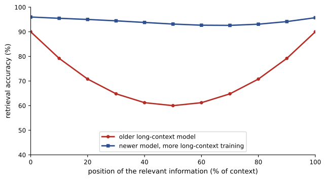
Using these methods, context windows of 128,000 tokens became common in 2024, and several models now accept a million tokens or more. A model accepting long inputs is not the same as a model using them well, however. Studies have found that models often retrieve information placed at the beginning or end of a long context more reliably than information in the middle, a pattern sometimes called lost in the middle. Simple tests such as finding one planted sentence in a long document (needle in a haystack) are now passed by most frontier models, so harder benchmarks test multi-step reasoning over many scattered facts.
Long context versus retrieval
A long context window and retrieval-augmented generation (Lesson 7) are two ways to give a model information it was not trained on. Long context is simple: put the whole document set in the prompt and let the model find what matters. Retrieval selects a few relevant passages first. The trade-offs are practical:
| Consideration | Long context | Retrieval |
|---|---|---|
| Setup | Minimal | Needs indexing, chunking and a retriever |
| Cost per query | High: every token is processed each time (reduced by prompt caching) | Low: only selected passages are processed |
| Latency | Grows with context length | Short prompts, plus retrieval time |
| Information across many documents | Can reason over everything at once | Limited to what the retriever finds |
| Very large collections | Impossible beyond the window | Scales to millions of documents |
| Failure mode | Missing details in the middle | Retriever misses the relevant passage |
Many applications combine them: retrieval narrows a large collection to a few dozen documents, which then fit comfortably in a long context. Prompt caching, offered by most commercial model providers, stores the KV cache of a repeated prompt prefix (such as a long instruction document) so that later requests reuse it at a fraction of the cost.
Inside attention: what heads learn
Research on trained models has identified attention patterns with recognizable functions. Induction heads, found in small and large models alike, look for an earlier occurrence of the current token and attend to the token that followed it, predicting that the pattern will repeat; they appear to underpin much of a model's ability to learn from examples in its prompt. Other heads attend mostly to the first token of the sequence, using it as a default place to put attention when nothing else is relevant, a phenomenon known as an attention sink; streaming methods that drop old tokens from the cache keep these first tokens for this reason. Such findings come from the field of mechanistic interpretability, discussed further in AI-430.
Common mistakes
MistakeAssuming attention knows token order without position information.
InsteadAttention is order-blind; positions must be encoded, usually with RoPE.
MistakeEstimating serving memory from the weights alone.
InsteadAdd the KV cache, which grows with context length and batch size.
MistakeAssuming a model with a long context window uses all of it reliably.
InsteadTest retrieval and reasoning across positions; performance can drop in the middle.
MistakeThinking FlashAttention approximates attention.
InsteadIt computes exact attention with less memory traffic.
MistakeChoosing long context or retrieval as if they were exclusive.
InsteadCombine them: retrieve to narrow, then use the long context.
Summary and key terms
- Causal self-attention weights earlier tokens by softmax of scaled query-key dot products.
- Attention costs grow quadratically with sequence length and are blind to order.
- RoPE rotates queries and keys so scores depend only on relative position.
- The KV cache stores keys and values for generation; its size grows with layers, KV heads, context and batch.
- MQA, GQA, latent attention and sliding windows shrink the cache.
- FlashAttention computes exact attention with tiling; linear-time layers offer alternatives.
- Context extension rescales RoPE frequencies and adds long-document training; long context and retrieval complement each other.
- Causal mask
- A rule preventing attention to later positions.
- Rotary position embedding (RoPE)
- Position encoding that rotates query and key pairs by position-dependent angles.
- KV cache
- Stored keys and values of earlier tokens used during generation.
- Grouped-query attention (GQA)
- Attention in which groups of query heads share key-value heads.
- Multi-query attention (MQA)
- Attention in which all query heads share one key-value head.
- Sliding-window attention
- Attention limited to a fixed number of recent tokens.
- FlashAttention
- A tiled algorithm computing exact attention with reduced memory traffic.
- State space model
- A sequence layer with a fixed-size recurrent state and linear cost.
- Position interpolation
- Scaling positions so a longer context maps into the trained range.
- Induction head
- An attention head that continues patterns seen earlier in the context.
Practice problems
Work each problem on paper first, then reveal the answer to check.
Why does attention need explicit position information?
Show answer
Its weighted sum is unchanged if tokens are reordered.
What property makes RoPE a relative position scheme?
Show answer
The score depends only on the difference between positions.
A model has 32 layers, 8 KV heads of dimension 128. KV cache for 32,000 tokens in 16 bits?
Show answer
2 × 32 × 8 × 128 × 32,000 × 2 = 4.2 GB.
By what factor does GQA with 8 KV heads reduce the cache compared with 64-head MHA?
Show answer
8.
Why does a sliding window cap the KV cache?
Show answer
Only the most recent window of tokens is kept.
What does FlashAttention reduce?
Show answer
Memory traffic, by not writing the full score matrix to main memory.
Why do pure state space models struggle with some tasks?
Show answer
Their fixed-size state makes exact recall of distant details hard.
How does position interpolation extend context?
Show answer
It scales positions down so long sequences fall in the trained range.
What is the lost-in-the-middle effect?
Show answer
Information in the middle of a long context is retrieved less reliably.
Give one advantage of retrieval over long context.
Show answer
Lower cost per query or scaling to collections larger than any window.
Lesson quiz · 5 questions
Score 60% or more to complete this lesson.
Create a free account to save your progress, take quizzes and earn a certificate.