Embeddings, contrastive learning and vector search

Generative models produce text and images, but many of the most useful AI systems never generate anything. Search engines, recommendation systems, duplicate detectors, clustering tools and the retrieval step of retrieval-augmented generation (Lesson 7) all depend on embeddings: vectors that represent the meaning of a piece of text, an image or a sound, arranged so that similar things are close together. Embeddings also connect the different parts of generative systems, linking text prompts to images in diffusion models (Lesson 9) and images to language in multimodal models. This lesson explains what embeddings are, how contrastive learning produces them, how models such as CLIP align images and text, how text embedding models are trained and evaluated, how vector search finds nearest neighbors among millions of items quickly, and the pitfalls of using embeddings in practice.

What an embedding is

An embedding maps an input to a vector of a few hundred to a few thousand numbers. The individual numbers have no fixed meaning; what matters is geometry. Inputs with similar meaning should have vectors pointing in similar directions, and similarity is usually measured by cosine similarity, the dot product of two vectors divided by the product of their lengths:

which ranges from -1 to 1. If vectors are normalized to unit length, cosine similarity is simply the dot product, and ranking by it is equivalent to ranking by Euclidean distance.

Word embeddings such as word2vec (2013) assigned one vector to each word, learned by predicting words from their neighbors; they famously captured analogies such as king minus man plus woman being close to queen. Language models produce contextual embeddings, in which the same word gets different vectors in different sentences, so "bank" in "river bank" and "bank account" are distinguished. For search and retrieval, what is usually needed is one vector for a whole sentence, passage or document, produced by a model trained specifically for that purpose.

Contrastive learning

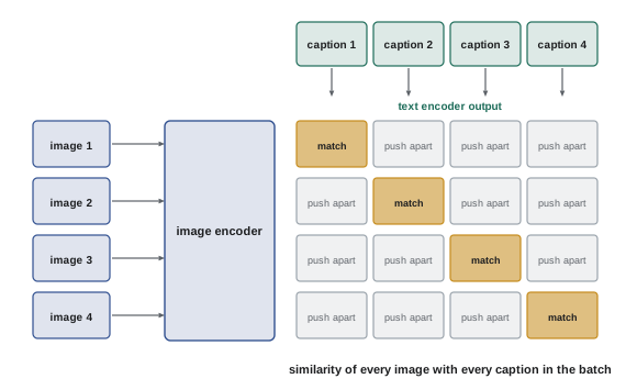
Contrastive learning trains an encoder by showing it pairs that should be similar (positives) and pairs that should not (negatives). A positive pair might be a question and the passage that answers it, two crops of the same photograph, or an image and its caption. Negatives are other items, conveniently the other examples in the same training batch (in-batch negatives). The most common objective, InfoNCE, treats each example as a classification problem: given an anchor, identify its positive among all the candidates in the batch. For anchor \(a_i\) with positive \(b_i\) and a batch of \(N\) candidates:

where \(\tau\) is a temperature that controls how sharply the loss focuses on the most similar candidates. Minimizing the loss pulls positives together and pushes negatives apart. Larger batches provide more negatives and generally produce better embeddings, and hard negatives, examples that look similar but are not true matches (a passage about the right topic that does not answer the question), are especially valuable.

CLIP: aligning images and text

In 2021, OpenAI released CLIP (Contrastive Language-Image Pre-training), trained with a symmetric InfoNCE loss on about 400 million image-caption pairs collected from the web. CLIP has two encoders, one for images and one for text, trained so that each image's embedding is closest to its own caption's embedding among all captions in a batch of tens of thousands, and vice versa. The result is a shared embedding space for images and language.

This space enables zero-shot classification: to classify an image among categories the model was never explicitly trained on, embed a text prompt for each category ("a photo of a dog", "a photo of a cat") and choose the category whose embedding is closest to the image's. CLIP-style encoders became building blocks throughout generative AI, guiding text-to-image models, serving as the vision encoders of multimodal language models, and filtering and captioning training data.

import numpy as np

# Contrastive (CLIP-style) learning signal and zero-shot classification on toy embeddings
rng = np.random.default_rng(3)
d, n = 64, 8
concepts = rng.normal(size=(n, d))                 # hidden meaning of 8 image-caption pairs
img = concepts + 0.6 * rng.normal(size=(n, d))     # image encoder output (noisy view)
txt = concepts + 0.6 * rng.normal(size=(n, d))     # text encoder output (another noisy view)

def normalize(v):
    return v / np.linalg.norm(v, axis=1, keepdims=True)

def info_nce(a, b, tau):
    logits = normalize(a) @ normalize(b).T / tau   # cosine similarities divided by temperature
    logits -= logits.max(axis=1, keepdims=True)
    logp = logits - np.log(np.exp(logits).sum(axis=1, keepdims=True))
    return -np.mean(np.diag(logp))                 # correct pair is on the diagonal

for tau in (1.0, 0.1, 0.03):
    loss = 0.5 * (info_nce(img, txt, tau) + info_nce(txt, img, tau))
    print(f"temperature {tau:<4}: symmetric InfoNCE loss {loss:.3f} (random guessing: {np.log(n):.3f})")
shuffled = txt[rng.permutation(n)]
print(f"mismatched pairs at temperature 0.1: loss {0.5 * (info_nce(img, shuffled, 0.1) + info_nce(shuffled, img, 0.1)):.3f}")

# Zero-shot classification: embed new images, pick the class whose text embedding is most similar
labels = 8
class_txt = concepts[:labels] + 0.6 * rng.normal(size=(labels, d))
correct = 0
trials = 400
for _ in range(trials):
    c = rng.integers(labels)
    new_img = concepts[c] + 3.5 * rng.normal(size=d)
    sims = normalize(class_txt) @ (new_img / np.linalg.norm(new_img))
    correct += int(np.argmax(sims) == c)
print(f"zero-shot accuracy on {labels} classes: {correct / trials:.1%} (chance {1 / labels:.1%})")

temperature 1.0 : symmetric InfoNCE loss 1.461 (random guessing: 2.079)
temperature 0.1 : symmetric InfoNCE loss 0.009 (random guessing: 2.079)
temperature 0.03: symmetric InfoNCE loss 0.000 (random guessing: 2.079)
mismatched pairs at temperature 0.1: loss 5.531
zero-shot accuracy on 8 classes: 70.5% (chance 12.5%)

The output shows that correctly matched pairs give a loss far below the value for random guessing (the logarithm of the batch size), and that mismatched pairs give a much higher loss, which is the signal that drives training. Lower temperatures sharpen the distinction. Zero-shot classification works well above chance even when the new images are much noisier than those seen in training.

Text embedding models

Modern text embedding models start from a pretrained language model and are fine-tuned contrastively in stages: first on large numbers of weakly related pairs mined from the web (titles and bodies, questions and answers, linked pages), then on smaller curated datasets with hard negatives, and often with instructions that tell the model what kind of similarity matters ("represent this query for retrieving supporting documents"). Embeddings are produced by averaging the final hidden states over the tokens or by using a special token's state.

The Massive Text Embedding Benchmark (MTEB), introduced in 2022, evaluates embedding models across retrieval, classification, clustering, semantic similarity and other tasks in many languages, and its leaderboard is the usual starting point for choosing a model. As with all benchmarks (Lesson 6), the best general model is not necessarily the best for a particular domain, and a small evaluation set of real queries is the most reliable guide.

Two practical choices affect cost. Larger embeddings capture more detail but take more storage and slower search; Matryoshka representation learning trains embeddings so that their first 64, 128 or 256 dimensions also work as smaller embeddings, letting users trade accuracy for size after training. And embeddings can be quantized, like model weights (Lesson 8), to 8 bits or even 1 bit per dimension for a first-pass search.

An embedding model that encodes queries and documents separately is called a bi-encoder. Its advantage is that document embeddings can be computed once and stored. A cross-encoder instead reads the query and a document together and outputs a relevance score; it is more accurate, because it can compare every word of the query with every word of the document, but far too slow to apply to millions of documents. Retrieval systems therefore use a bi-encoder to retrieve a few hundred candidates and a cross-encoder to rerank them.

Vector search

Finding the items most similar to a query is a nearest-neighbor search. Exact search compares the query with every stored vector, which takes time proportional to the size of the collection: acceptable for thousands of items, but too slow for hundreds of millions under a latency budget of tens of milliseconds. Approximate nearest-neighbor (ANN) methods trade a small loss of recall, the fraction of true nearest neighbors found, for large speedups:

• Inverted file (IVF) indexes cluster the vectors with k-means and, at query time, search only the vectors in the few clusters whose centers are closest to the query.
• Graph indexes such as HNSW (hierarchical navigable small world) link each vector to its near neighbors in a multi-layer graph and find nearest neighbors by greedy navigation from coarse to fine layers. They offer excellent speed and recall at the cost of memory for the graph.
• Product quantization compresses vectors by splitting them into sub-vectors and replacing each with the index of the nearest entry in a small codebook, so that billions of vectors fit in memory and distances can be estimated from lookup tables.

import numpy as np

# Approximate search for the closest vectors with an inverted file (IVF) index
rng = np.random.default_rng(0)
n, d, k = 50_000, 64, 10
seeds = rng.normal(size=(2000, d)) * 1.5
X = seeds[rng.integers(0, 2000, n)] + rng.normal(size=(n, d))
X /= np.linalg.norm(X, axis=1, keepdims=True)
Q = X[rng.integers(0, n, 100)] + 0.1 * rng.normal(size=(100, d))
Q /= np.linalg.norm(Q, axis=1, keepdims=True)

def topk(scores, k):
    idx = np.argpartition(-scores, k)[:k]
    return idx[np.argsort(-scores[idx])]

truth = [set(topk(X @ q, k)) for q in Q]

# Build the index: k-means into nlist cells (a few iterations)
nlist = 256
C = X[rng.choice(n, nlist, replace=False)]
for _ in range(8):
    assign = np.argmax(X @ C.T, axis=1)
    for j in range(nlist):
        m = X[assign == j]
        if len(m):
            C[j] = m.mean(axis=0) / np.linalg.norm(m.mean(axis=0))
cells = [np.where(assign == j)[0] for j in range(nlist)]

for nprobe in (1, 4, 16, 64):
    hits, scanned = 0, 0
    for q, t in zip(Q, truth):
        probe = topk(C @ q, nprobe)
        cand = np.concatenate([cells[j] for j in probe])
        scanned += len(cand)
        found = cand[topk(X[cand] @ q, min(k, len(cand) - 1))]
        hits += len(t & set(found))
    print(f"nprobe {nprobe:3d}: recall@{k} {hits / (k * len(Q)):.3f}, "
          f"vectors scanned {scanned / len(Q) / n:.1%} of the collection")

nprobe   1: recall@10 0.536, vectors scanned 0.4% of the collection
nprobe   4: recall@10 0.749, vectors scanned 1.6% of the collection
nprobe  16: recall@10 0.888, vectors scanned 6.3% of the collection
nprobe  64: recall@10 0.984, vectors scanned 24.9% of the collection

Searching only the single closest cluster scans less than half a percent of the vectors but finds only about half the true nearest neighbors, because many lie near cluster boundaries. Searching 16 clusters raises recall to about 89 percent while scanning 6 percent of the collection, and 64 clusters gives 98 percent recall at a quarter of the cost of exact search. Production systems tune this trade-off to their latency budget and quality needs. Libraries such as FAISS and vector databases implement these indexes, often with filters (for example, restricting results to documents a user is permitted to see) and hybrid search that combines vector similarity with traditional keyword scoring such as BM25, which remains better at matching rare terms, names and codes exactly.

Uses of embeddings

Beyond retrieval for language models, embeddings support:

• Semantic search, which finds documents that match the meaning of a query even when they use different words.
• Recommendation, by embedding users and items in the same space.
• Clustering and topic discovery in large collections of documents or customer feedback.
• Deduplication of near-identical content, complementing the MinHash methods of Lesson 4.
• Classification with few labels, by training a simple classifier on top of embeddings.
• Anomaly detection, by flagging items far from any cluster of normal examples.

Pitfalls

Embeddings are powerful but imperfect:

• Domain shift. A general-purpose model may not separate concepts that matter in a specialized field, such as two legal doctrines or two part numbers, and may need fine-tuning on domain pairs.
• Negation and numbers. Embeddings often place "the drug is safe for children" close to "the drug is not safe for children", and handle quantities poorly, so they should not be relied upon for distinctions of this kind without reranking or other checks.
• Bias. Embeddings learned from human text reflect its associations. A 2016 study showed that word embeddings associated occupations with gender stereotypes, and similar effects appear in modern sentence and image embeddings, affecting search and recommendation results.
• Privacy. Embeddings are not anonymized data. Research published in 2023 showed that much of the original text can be reconstructed from its embedding, so embeddings of confidential or personal text must be protected like the text itself.
• Version lock-in. Embeddings from different models, or different versions of the same model, are not comparable, so changing the model means re-embedding the whole collection.