
STAT-235 · Lesson 9 of 12 · 26 min
Analysis of variance and design of experiments
Lesson 7 compared two means with a t test. Engineering experiments usually compare more: three curing methods, four suppliers, five mix designs. And they often vary several factors at once, such as the temperature, pressure and time of a welding process, because the factors may interact. Running many separate t tests inflates the chance of false alarms (Lesson 8) and wastes data. The analysis of variance (ANOVA) compares several means in one test by splitting the total variation in the data into parts due to the factors and a part due to random error. This lesson develops one-way ANOVA and the follow-up comparisons that say which means differ, extends it to blocked designs, and then introduces factorial experiments, the efficient way to study several factors and their interactions, putting into practice the design principles of Lesson 2.
One-way analysis of variance
Suppose k treatments are compared, with \(n_i\) observations on treatment i, treatment means \(\bar{y}_i\) and overall mean \(\bar{y}\). Each observation's deviation from the overall mean splits into a between-treatment part and a within-treatment part, and the sums of squares add:
Dividing each sum of squares by its degrees of freedom (k − 1 for treatments and N − k for error, where N is the total number of observations) gives mean squares. The error mean square estimates the random variance σ² whatever the treatment means are; the treatment mean square estimates σ² only if all treatment means are equal, and is larger otherwise. Their ratio is the test statistic:
Under the null hypothesis that all means are equal, F follows an F distribution with k − 1 and N − k degrees of freedom (Lesson 6). Large values of F are evidence that at least one mean differs.
Worked problem
Comparing three curing methods
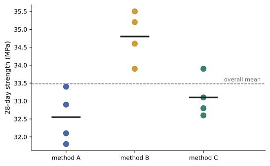
Four concrete cylinders were cured by each of three methods. The 28-day strengths (MPa) were A: 32.1, 33.4, 31.8, 32.9; B: 34.6, 35.2, 33.9, 35.5; C: 32.8, 33.9, 33.1, 32.6. Do the methods differ?
Show solution
- Treatment means: 32.55, 34.80, 33.10; overall mean 33.48.
- \(SS_{treatments} = 4[(-0.93)^2 + (1.32)^2 + (-0.38)^2] = 11.01\) with 2 degrees of freedom: \(MS = 5.50\).
- \(SS_{error}\) = 1.61 + 1.50 + 0.98 = 4.09 (squared deviations within each method) with 9 degrees of freedom: \(MS = 0.454\).
- \(F = 5.50/0.454 = 12.1\); the 5% critical value of \(F_{2,9}\) is 4.26, and p = 0.003.
Answer: The curing methods differ significantly (F = 12.1, p = 0.003). ANOVA says only that not all means are equal; the follow-up comparisons below identify which ones differ.
| Source | SS | df | MS | F | p |
|---|---|---|---|---|---|
| Curing method | 11.01 | 2 | 5.50 | 12.1 | 0.003 |
| Error | 4.09 | 9 | 0.454 | ||
| Total | 15.10 | 11 |
Which means differ?
After a significant F test, the natural next question is which pairs of treatments differ. Comparing every pair with ordinary t tests reintroduces the multiple-comparison problem. Tukey's honestly significant difference (HSD) method compares all pairs while holding the overall chance of any false alarm at the chosen level. Planned comparisons decided before seeing the data, such as each new method against a standard, can use more powerful methods.
from scipy import stats

A = [32.1, 33.4, 31.8, 32.9]     # 28-day strength (MPa), curing method A
B = [34.6, 35.2, 33.9, 35.5]     # method B
C = [32.8, 33.9, 33.1, 32.6]     # method C

F, p = stats.f_oneway(A, B, C)
print(f"One-way ANOVA: F = {F:.2f}, p = {p:.4f}")
res = stats.tukey_hsd(A, B, C)
names = "ABC"
for i in range(3):
    for j in range(i + 1, 3):
print(f" {names[i]} vs {names[j]}: difference {sum([A, B, C][i]) / 4 - sum([A, B, C][j]) / 4:+.2f} MPa, Tukey p = {res.pvalue[i, j]:.3f}")One-way ANOVA: F = 12.11, p = 0.0028 A vs B: difference -2.25 MPa, Tukey p = 0.003 A vs C: difference -0.55 MPa, Tukey p = 0.508 B vs C: difference +1.70 MPa, Tukey p = 0.015
Method B gives significantly higher strength than both A and C, by about 2.3 and 1.7 MPa, while A and C cannot be distinguished. An engineer would now ask whether B's advantage justifies its cost, and whether it holds across cement batches, which calls for a blocked design.
Assumptions and checks
ANOVA assumes independent observations, roughly normal errors and similar variances in all groups. Independence comes from randomization (Lesson 2). The other two are checked with the residuals \(y_{ij} - \bar{y}_i\): a normal probability plot of the residuals should be roughly straight, and plotting the residuals by group or against the fitted values should show similar spread. ANOVA is fairly robust to mild non-normality and, with equal group sizes, to moderately unequal variances. When the assumptions fail badly, a transformation (such as taking logarithms of skewed data) or the rank-based Kruskal-Wallis test can be used.
Blocking and two-way ANOVA
Lesson 2 designed the curing experiment in blocks: each day's cement batch was split among the methods. In the analysis, a block term is added, so the total sum of squares splits into treatments, blocks and error. Because batch-to-batch variation is removed from the error, the test for treatments becomes much more sensitive, the same idea as the paired t test, extended to more than two treatments. More generally, two-way ANOVA studies two factors at once, such as curing method and cement type, and, if the experiment is replicated, tests whether they interact. That leads to factorial designs.
Factorial experiments
A factorial experiment runs every combination of the levels of several factors. The most widely used are \(2^k\) designs, with each of k factors at a low and a high level, coded −1 and +1. They have two great advantages over changing one factor at a time. First, every run contributes to the estimate of every factor's effect, so they are far more efficient. Second, they reveal interactions: whether the effect of one factor depends on the level of another. One-factor-at-a-time experiments cannot detect interactions, and when interactions exist they can point to a poor optimum.
The main effect of a factor is the average response at its high level minus the average at its low level. The interaction effect of two factors is half the difference between the effect of one factor at the high and at the low level of the other.
Worked problem
Surface finish in machining
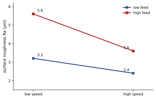
A 2² experiment measured surface roughness (µm, lower is better) at two cutting speeds and two feed rates: low speed and low feed 3.2; high speed and low feed 2.4; low speed and high feed 5.6; high speed and high feed 3.6. Estimate the effects.
Show solution
- Speed effect: average at high speed minus average at low speed: \((2.4 + 3.6)/2 - (3.2 + 5.6)/2 = 3.0 - 4.4 = -1.4\).
- Feed effect: \((5.6 + 3.6)/2 - (3.2 + 2.4)/2 = 4.6 - 2.8 = 1.8\).
- Speed effect at low feed: 2.4 − 3.2 = −0.8; at high feed: 3.6 − 5.6 = −2.0. Interaction: \((-2.0 - (-0.8))/2 = -0.6\).
Answer: Higher speed improves the finish (−1.4 µm) and higher feed worsens it (+1.8 µm), and the benefit of high speed is larger at high feed: an interaction of −0.6 µm. So if productivity requires the high feed, the high speed is especially important. With single runs there is no estimate of error, so replicates (or the pooling methods below) are needed before declaring effects significant.
A replicated 2³ experiment
With replicates, each effect can be tested. In a \(2^k\) design with N runs in total and pooled replicate variance \(s^2\), each effect has standard error \(2s/\sqrt{N}\), and dividing an effect by its standard error gives a t statistic. The code evaluates a welding experiment with temperature, pressure and time each at two levels, run twice in random order.
import itertools
import numpy as np
from scipy import stats

# 2^3 factorial, two replicates: weld strength (MPa) for A = temperature, B = pressure, C = time
runs = list(itertools.product([-1, 1], repeat=3))           # (A, B, C) in coded units
y = np.array([[41.2, 42.0], [44.8, 45.9], [47.1, 46.0], [53.9, 55.2],
              [41.9, 41.4], [45.3, 46.6], [46.8, 47.9], [55.0, 54.1]])
X = np.array(runs)
ybar = y.mean(axis=1)
N = y.size
s2 = np.mean(y.var(axis=1, ddof=1))                         # pooled replicate variance
se = 2 * np.sqrt(s2 / N)                                    # standard error of an effect
dof = N - len(runs)
cols = {"A": X[:, 0], "B": X[:, 1], "C": X[:, 2],
        "AB": X[:, 0] * X[:, 1], "AC": X[:, 0] * X[:, 2], "BC": X[:, 1] * X[:, 2],
        "ABC": X[:, 0] * X[:, 1] * X[:, 2]}
print(f"Standard error of each effect: {se:.2f} MPa ({dof} df)")
for name, c in cols.items():
    effect = 2 * np.mean(c * ybar)
    p = 2 * stats.t.sf(abs(effect / se), dof)
    flag = "  significant" if p < 0.05 else ""
    p_text = "< 0.0001" if p < 1e-4 else f"= {p:.4f}"
print(f"{name:3s} effect {effect:+6.2f} MPa p {p_text}{flag}")Standard error of each effect: 0.37 MPa (8 df) A effect +0.36 MPa p = 0.3546 B effect +7.11 MPa p < 0.0001 significant C effect +5.81 MPa p < 0.0001 significant AB effect +0.04 MPa p = 0.9215 AC effect -0.06 MPa p = 0.8697 BC effect +1.79 MPa p = 0.0013 significant ABC effect -0.34 MPa p = 0.3870
Pressure and time both raise weld strength strongly, and they interact: longer time helps more at high pressure. Temperature, within the range tested, has no detectable effect, which is useful knowledge too, since it can be set for cost or convenience. Sixteen runs gave precise estimates of all three main effects and every interaction, something no one-factor-at-a-time plan of the same size could do.
Beyond the basics
With many factors, a full factorial becomes large: 7 factors at two levels need 128 runs. Fractional factorial designs run a carefully chosen fraction, such as 16 of the 128, accepting that some high-order interactions (usually negligible) are confounded with main effects. They are ideal for screening many candidate factors to find the few that matter. Once the important factors are known, response surface methods fit curved models, using designs with three or more levels, to locate an optimum. These methods, together with the robust design ideas of Taguchi, are central to process development and quality improvement in manufacturing, chemical processing and materials engineering.
Common mistakes
MistakeComparing several means with many separate t tests.
InsteadUse ANOVA, then a multiple-comparison method such as Tukey's HSD.
MistakeConcluding from a significant F that every mean differs.
InsteadF shows that at least one differs; follow-up comparisons say which.
MistakeSkipping residual checks.
InsteadCheck normality and equal spread with residual plots.
MistakeStudying factors one at a time.
InsteadUse factorial designs, which are more efficient and reveal interactions.
MistakeInterpreting main effects alone when a strong interaction exists.
InsteadDescribe each factor's effect at each level of the interacting factor.
Summary and key terms
- ANOVA splits total variation into treatment and error sums of squares.
- F = MS_treatments/MS_error, with k − 1 and N − k degrees of freedom, tests equality of k means.
- Tukey's HSD compares all pairs while controlling the overall false-alarm rate.
- Residual plots check the normality and equal-variance assumptions.
- Blocking removes known nuisance variation and sharpens comparisons.
- 2ᵏ factorial designs estimate all main effects and interactions efficiently.
- An interaction means the effect of one factor depends on another; fractional factorials screen many factors cheaply.
- Analysis of variance
- Testing equality of several means by partitioning variation.
- Sum of squares
- A total of squared deviations, partitioned among sources of variation.
- Mean square
- A sum of squares divided by its degrees of freedom.
- ANOVA table
- A summary of sums of squares, degrees of freedom, mean squares and F tests.
- Tukey's HSD
- A method for comparing all pairs of means with controlled overall error.
- Kruskal-Wallis test
- A rank-based alternative to one-way ANOVA.
- Factorial design
- An experiment that runs every combination of factor levels.
- Main effect
- The average change in response when a factor moves from low to high.
- Interaction
- A dependence of one factor's effect on the level of another.
- Fractional factorial
- A design using a planned fraction of the full factorial runs.
Practice problems
Work each problem on paper first, then reveal the answer to check.
An experiment has 5 treatments with 6 observations each. Give the degrees of freedom for treatments, error and total.
Show answer
4, 25 and 29.
If SS_treatments = 40 and SS_error = 50 in that experiment, find F.
Show answer
MS = 10 and 2; F = 5.0.
Is F = 5.0 with (4, 25) df significant at 5% (critical value 2.76)?
Show answer
Yes.
Why does SS_error not depend on whether the treatment means are equal?
Show answer
It measures variation within groups, around each group's own mean.
What does a straight normal probability plot of residuals indicate?
Show answer
The normality assumption is reasonable.
How many runs does a full 2⁴ factorial need, and a half fraction?
Show answer
16 and 8.
In a 2² design, (1) = 10, a = 14, b = 12, ab = 20. Find the A effect.
Show answer
(14 + 20)/2 − (10 + 12)/2 = 6.
Find the AB interaction for that design.
Show answer
A effect at high B: 8; at low B: 4; interaction (8 − 4)/2 = 2.
A replicated 2³ design has 16 runs and s = 1.2. Find the standard error of an effect.
Show answer
2 × 1.2/4 = 0.6.
Why can a one-factor-at-a-time study miss the optimum?
Show answer
It cannot detect interactions, so the best level of one factor may depend on another.
Lesson quiz · 5 questions
Score 60% or more to complete this lesson.
Create a free account to save your progress, take quizzes and earn a certificate.