More inference: variances, proportions, counts and resampling

Lesson 7 built confidence intervals and hypothesis tests for means and for a single proportion. Engineering questions often concern other quantities. Is a filling machine consistent enough, regardless of its average? Is one supplier's defect rate really higher than another's? Are defects spread evenly across shifts, or do they cluster? Does the failure mode depend on the supplier? What if the data are skewed, ranked or too few for normal-theory methods? This lesson extends inference to variances (with the chi-square and F distributions of Lesson 6), to comparisons of two proportions, to counts in categories (chi-square goodness-of-fit and contingency tests), to methods that do not assume normality (nonparametric tests and the bootstrap), and to the pitfalls of running many tests at once. Throughout, the logic is the same as in Lesson 7: a test statistic, its distribution if the null hypothesis is true, and a p-value or interval interpreted in engineering terms.

Inference about a variance

Uniformity is often as important as the average: the fill weight of packages, the thickness of a coating, the diameter of a shaft, the strength of a batch of concrete. For a sample of size n from a normal population, \((n - 1)S^2/\sigma^2\) has a chi-square distribution with n − 1 degrees of freedom (Lesson 6), which gives a confidence interval for σ²:

where \(\chi^2_{\alpha/2}\) is the upper critical value (the larger one). Because the chi-square distribution is skewed, the interval is not symmetric about \(s^2\). Taking square roots gives an interval for σ.

Comparing two variances

To compare the variability of two independent normal populations, use the ratio \(F = s_1^2/s_2^2\), which follows an F distribution with \(n_1 - 1\) and \(n_2 - 1\) degrees of freedom when \(\sigma_1 = \sigma_2\). By convention the larger variance goes on top, and the test is two-sided unless there is a prior reason to expect one process to be more variable.

Comparing two proportions

To compare the proportions of items with some property in two populations, such as defective parts from two suppliers or failures under two designs, use the difference of sample proportions \(\hat{p}_1 - \hat{p}_2\). Under the null hypothesis \(p_1 = p_2\), the pooled proportion \(\hat{p} = (x_1 + x_2)/(n_1 + n_2)\) estimates the common value, and

is approximately standard normal when each sample contains at least about 10 items with and 10 without the property.

Counts in categories: chi-square tests

Goodness of fit

When observations fall into k categories, the chi-square goodness-of-fit test checks whether the observed counts \(O_i\) are consistent with expected counts \(E_i\) from a hypothesized model:

Large values mean poor agreement. If the model is correct, the statistic has approximately a chi-square distribution with k − 1 degrees of freedom, minus one more for each parameter estimated from the data. The approximation needs expected counts of at least about 5 in each category; combine sparse categories if necessary. The test can check whether defects are spread evenly over shifts, machines or days, or whether failure counts follow a Poisson distribution (Lesson 4).

Contingency tables

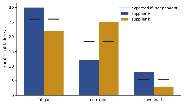
When each item is classified by two categorical variables, such as failure mode and supplier, or defect type and production line, the counts form a contingency table. The chi-square test of independence asks whether the two classifications are related. The expected count for each cell, if they are independent, is (row total × column total)/grand total, and the statistic has (rows − 1) × (columns − 1) degrees of freedom. The code below runs the tests of this lesson.

import numpy as np
from scipy import stats

# F test: are two filling machines equally consistent?
s1, n1, s2, n2 = 3.1, 10, 1.9, 12
F = s1**2 / s2**2
p = 2 * min(stats.f.sf(F, n1 - 1, n2 - 1), stats.f.cdf(F, n1 - 1, n2 - 1))
print(f"F = {F:.2f} with ({n1 - 1}, {n2 - 1}) df, two-sided p = {p:.3f}")

# Two proportions: defect rates from two suppliers
x = np.array([18, 7]); n = np.array([400, 350])
pool = x.sum() / n.sum()
z = (x[0] / n[0] - x[1] / n[1]) / np.sqrt(pool * (1 - pool) * (1 / n[0] + 1 / n[1]))
print(f"Defect rates {x[0] / n[0]:.3f} vs {x[1] / n[1]:.3f}: z = {z:.2f}, two-sided p = {2 * stats.norm.sf(abs(z)):.3f}")

# Chi-square goodness of fit: defects by shift, equal production on each shift
obs = [45, 38, 67]
chi2, p = stats.chisquare(obs)
print(f"Defects by shift {obs}: chi-square = {chi2:.2f}, p = {p:.4f}")

# Contingency table: failure mode by supplier
table = np.array([[30, 12, 8],      # supplier A: fatigue, corrosion, overload
                  [22, 25, 3]])     # supplier B
chi2, p, dof, expected = stats.chi2_contingency(table)
print(f"Failure mode vs supplier: chi-square = {chi2:.2f}, {dof} df, p = {p:.4f}")

F = 2.66 with (9, 11) df, two-sided p = 0.129
Defect rates 0.045 vs 0.020: z = 1.90, two-sided p = 0.057
Defects by shift [45, 38, 67]: chi-square = 9.16, p = 0.0103
Failure mode vs supplier: chi-square = 8.07, 2 df, p = 0.0177

The two filling machines do not differ significantly in variability with these sample sizes (p = 0.13). The failure-mode table shows a significant association (p ≈ 0.02): supplier B's parts fail by corrosion far more often, a pointer to coating or material differences that a single overall failure rate would hide.

Nonparametric methods

The t tests of Lesson 7 assume roughly normal data, an assumption that matters most for small samples. When data are strongly skewed, contain outliers, or are only ranks (such as condition ratings from 1 to 5), nonparametric (distribution-free) methods are safer. They work with signs or ranks rather than the values themselves:

• The sign test checks whether the median equals a hypothesized value by counting observations above and below it; under the null hypothesis the count is binomial with p = 0.5 (Lesson 4).
• The Wilcoxon signed-rank test, for paired data or a single median, uses the ranks of the absolute differences and is more powerful than the sign test.
• The Mann-Whitney (Wilcoxon rank-sum) test compares two independent samples by ranking all observations together, the nonparametric counterpart of the two-sample t test.

These tests lose a little power when the data really are normal, typically requiring about 5% more observations, but they can be far more reliable when they are not.

The bootstrap

For many statistics, such as a median, a percentile, a ratio or a correlation, there is no convenient formula for the standard error. The bootstrap estimates it by resampling: treat the sample as a stand-in for the population, draw many new samples of the same size from it with replacement, compute the statistic for each, and use the spread of these bootstrap values as a measure of uncertainty. The 2.5th and 97.5th percentiles of the bootstrap values give a simple 95% interval (the percentile method). The method needs no distributional assumptions, only that the sample is representative and the observations independent, and it is easy to apply to any statistic a computer can calculate.

import numpy as np

rng = np.random.default_rng(11)
# Repair times (hours) for 15 breakdowns: skewed, with one long job
times = np.array([0.8, 1.1, 1.3, 1.5, 1.6, 1.9, 2.0, 2.2, 2.4, 2.9, 3.3, 3.8, 4.6, 6.1, 14.5])
print(f"Sample median {np.median(times):.2f} h, sample mean {times.mean():.2f} h")

boot = [np.median(rng.choice(times, times.size, replace=True)) for _ in range(20000)]
lo, hi = np.percentile(boot, [2.5, 97.5])
print(f"Bootstrap 95% interval for the median: {lo:.2f} to {hi:.2f} h")

boot_mean = [rng.choice(times, times.size, replace=True).mean() for _ in range(20000)]
lo, hi = np.percentile(boot_mean, [2.5, 97.5])
print(f"Bootstrap 95% interval for the mean:   {lo:.2f} to {hi:.2f} h")

Sample median 2.20 h, sample mean 3.33 h
Bootstrap 95% interval for the median: 1.60 to 3.80 h
Bootstrap 95% interval for the mean:   2.01 to 5.26 h

The one 14.5-hour job pulls the mean up to 3.3 h and makes its interval wide and lopsided, while the median of 2.2 h is more stable. For planning typical repairs the median is the better summary; for total downtime cost the mean is what matters, and the bootstrap shows how uncertain it is.

Many tests, and what significance means

Each test at the 5% level has a 5% chance of a false alarm when there is no real effect. Run 20 independent tests and the chance of at least one false alarm is \(1 - 0.95^{20} = 0.64\). Searching through many variables, subgroups or outcomes for something significant, and reporting only what turns up, is called data dredging or p-hacking, and it produces findings that fail to replicate. Remedies include deciding the hypotheses before collecting data, adjusting the significance level (the Bonferroni correction tests each of m hypotheses at α/m), and confirming surprising results with new data.

Finally, statistical significance is not engineering significance. With enough data, a difference too small to matter becomes significant; with too little, an important difference may not. Always report the estimated size of the effect with a confidence interval, and judge it against what matters in practice: a tolerance, a cost, a safety margin.