
ROB-410 · Lesson 6 of 12 · 31 min
Reward design and safety in reinforcement learning
A reinforcement learning agent optimizes exactly what it is rewarded for, not what its designers meant. That simple fact explains a large share of failed robot learning projects. A reward that seems obviously right can lead to behaviour that technically scores well while missing the point entirely, and an agent that explores freely can damage itself, its surroundings or people. This lesson covers how to design rewards that produce the intended behaviour, how to recognize and prevent reward hacking, and how to keep learning robots safe during both training and deployment.
What a reward has to do
A reward function turns the designer's intentions into a number at every step. It has to do three jobs at once. It must define success correctly, so that the best-scoring behaviour is the behaviour you want. It should provide enough signal for learning to make progress, rather than leaving the agent wandering with no feedback. And it should discourage side effects that the designer cares about but did not think to mention, such as excessive force, jerky motion, energy waste or knocking other objects over.
Those goals pull against each other. A sparse reward of +1 for task success and 0 otherwise defines success precisely but gives almost no learning signal, as lesson 4 showed for random exploration. A dense reward with many terms gives plenty of signal but creates many opportunities for unintended trade-offs. Good reward design is the craft of finding the simplest reward that is both correct and learnable.
| Reward style | Example for grasp-and-lift | Advantages | Risks |
|---|---|---|---|
| Sparse | +1 when object held 10 cm above table for 2 s | Unambiguous, hard to exploit | Very slow learning |
| Dense distance-based | −distance(gripper, object) every step | Strong early signal | Robot hovers near object without grasping |
| Staged | Bonuses for reach, contact, lift, hold | Guides through phases | Agent may farm early stages |
| Potential-based shaping | \( \gamma \Phi(s') - \Phi(s) \) added to sparse reward | Speeds learning, keeps optimal policy | Needs a sensible potential function |
| Learned from people | Reward model trained on preferences or demonstrations | Captures hard-to-write goals | Model errors can be exploited |
Reward shaping
Shaping means adding intermediate rewards to guide learning. The danger is that the shaping terms change which behaviour is optimal. A classic illustration comes from simulated soccer: rewarding a robot for touching the ball produced an agent that vibrated against the ball to collect touch rewards rather than scoring. In manipulation, rewarding proximity to an object can produce an agent that hovers just above the object, because closing the gripper risks pushing the object away and losing proximity reward.
Potential-based shaping avoids this. Choose a potential function \( \Phi(s) \) that estimates how close a state is to success, such as the negative distance from gripper to object, and add the shaping term \( F(s, s') = \gamma \Phi(s') - \Phi(s) \) to the original reward. Over any trajectory, these terms telescope: their discounted sum depends only on the start and end states, not on the path. As a result, potential-based shaping provably leaves the optimal policy unchanged while giving the agent a helpful gradient towards success.
Worked problem
Why potential-based shaping cannot be farmed
A robot moves around a loop of states \( s_1 \to s_2 \to s_3 \to s_1 \) with potentials 2, 5 and 3, earning no task reward. With \( \gamma = 1 \), what total shaping reward does it collect per lap? What about a naive bonus of +1 every time it enters \( s_2 \)?
Show solution
- Shaping terms: \( (5-2) + (3-5) + (2-3) = 3 - 2 - 1 = 0 \).
- A full lap earns zero shaping reward, so looping gains nothing.
- The naive bonus pays +1 on every lap, forever.
- An agent maximizing the naive reward would circle the loop instead of finishing the task.
Answer: Zero per lap with potential-based shaping, but +1 per lap with the naive bonus. Potential differences cannot be farmed by going in circles.
# Potential-based shaping keeps the optimal policy; a naive bonus does not
import numpy as np
# Chain of 6 states, start at 0, goal at 5 (+10). Actions: 0 = left, 1 = right.
# State 2 has a "bonus" for naive shaping. Step cost -0.1.
N, gamma = 6, 0.95
def solve(shape):
    V = np.zeros(N)
    for _ in range(500):
        Vn = V.copy()
        for s in range(N - 1):
            qs = []
            for a in (0, 1):
                s2 = max(0, s - 1) if a == 0 else s + 1
                r = -0.1 + (10.0 if s2 == N - 1 else 0.0)
                if shape == 'naive' and s2 == 2:
                    r += 2.0                                     # bonus every visit to state 2
                if shape == 'potential':
                    phi = lambda x: 2.0 * x                      # closer to goal = higher potential
                    r += gamma * (0 if s2 == N - 1 else phi(s2)) - phi(s)
                qs.append(r + gamma * (0 if s2 == N - 1 else V[s2]))
            Vn[s] = max(qs)
        V = Vn
    pol = []
    for s in range(N - 1):
        qs = []
        for a in (0, 1):
            s2 = max(0, s - 1) if a == 0 else s + 1
            r = -0.1 + (10.0 if s2 == N - 1 else 0.0)
            if shape == 'naive' and s2 == 2: r += 2.0
            if shape == 'potential':
                r += gamma * (0 if s2 == N - 1 else 2.0 * s2) - 2.0 * s
            qs.append(r + gamma * (0 if s2 == N - 1 else V[s2]))
        pol.append('R' if qs[1] >= qs[0] else 'L')
    return ''.join(pol)
for shape in ('none', 'potential', 'naive'):
print(f"{shape:9s} optimal actions in states 0-4: {solve(shape)}")none optimal actions in states 0-4: RRRRR potential optimal actions in states 0-4: RRRRR naive optimal actions in states 0-4: RRRLL
Reward hacking and specification gaming
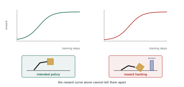
Reward hacking, also called specification gaming, happens when an agent finds a way to score highly that the designer did not intend. In simulation it is common and sometimes spectacular: agents exploit physics-engine bugs to move faster than intended, flip objects so that a sensor reading looks like success, or learn that ending an episode early avoids penalties. On real robots, hacking tends to be subtler: a policy that lifts the object briefly to trigger the success detector and then drops it, or one that pushes the object into the camera's blind spot where a detector reports it as removed.
Several habits catch hacking early. Watch videos of the learned behaviour regularly, not just the reward curve, because a rising return can hide degenerate behaviour. Make success detectors robust, for example by requiring an object to stay lifted for a few seconds and checking it with two independent signals. Add terms for side effects you care about, such as penalties on contact forces above a threshold or on large changes in action. Keep the simulator honest by randomizing physics, as lesson 7 describes, so that exploits that depend on exact parameters stop working. And evaluate in conditions that differ from training, since a policy that relies on a quirk will usually fail when the quirk is absent.
Worked problem
Diagnosing a suspicious success rate
A simulated wiping policy reaches a 98 % success rate, where success means the dirt-particle count on a table falls below 5 %. Videos show the sponge moving fast near the table edge. What might be happening, and how would you check?
Show solution
- A plausible hack is that particles are pushed off the table edge rather than wiped up, which still reduces the count on the table.
- Check by counting particles that leave the table area, and by logging where removed particles end up.
- Fix by defining success as particles absorbed by the sponge, or by penalizing particles pushed off the table.
- Re-evaluate on tables with raised edges or different sizes to see whether performance collapses.
Answer: The policy is probably exploiting the success definition. Measure what actually happens to the particles and redefine success so that pushing them away does not count.
Combining multiple objectives
Most real tasks have several objectives: complete the task, do it quickly, use little energy, keep forces low, move smoothly and avoid collisions. A weighted sum of terms is the usual approach, \( r = w_1 r_{\text{task}} - w_2 \|\tau\|^2 - w_3 \|a_t - a_{t-1}\|^2 - w_4 \cdot \text{collision} \), but the weights are hard to set. Too much weight on smoothness and the policy may freeze; too little and it may jitter in ways that wear out gearboxes. A practical procedure is to start with only the task term until the policy can sometimes succeed, then add penalty terms one at a time, checking behaviour after each. Normalizing each term by a typical value makes weights more interpretable.
When some requirements are hard limits rather than preferences, such as maximum contact force or minimum distance to a person, it is often better to express them as constraints rather than as penalties. Constrained RL methods optimize the task reward subject to the expected cost of constraint violations staying below a threshold. A common approach adds a Lagrange multiplier that grows automatically while the constraint is being violated and shrinks when it is satisfied, so the agent is pushed harder towards compliance only when needed.
Worked problem
A Lagrange multiplier update
A constrained RL agent must keep its average excessive-force cost per episode at or below \( d = 0.5 \). The multiplier \( \lambda \) starts at 1.0 and is updated by \( \lambda \gets \max(0, \lambda + \eta (\bar{c} - d)) \) with \( \eta = 0.5 \). Measured average costs over three updates are 1.3, 0.9 and 0.4. What is \( \lambda \) after each?
Show solution
- After 1.3: \( 1.0 + 0.5(1.3 - 0.5) = 1.4 \).
- After 0.9: \( 1.4 + 0.5(0.9 - 0.5) = 1.6 \).
- After 0.4: \( 1.6 + 0.5(0.4 - 0.5) = 1.55 \).
Answer: 1.4, 1.6 and 1.55. The penalty weight rose while the constraint was violated and began to fall once it was met.
Safe exploration on real robots
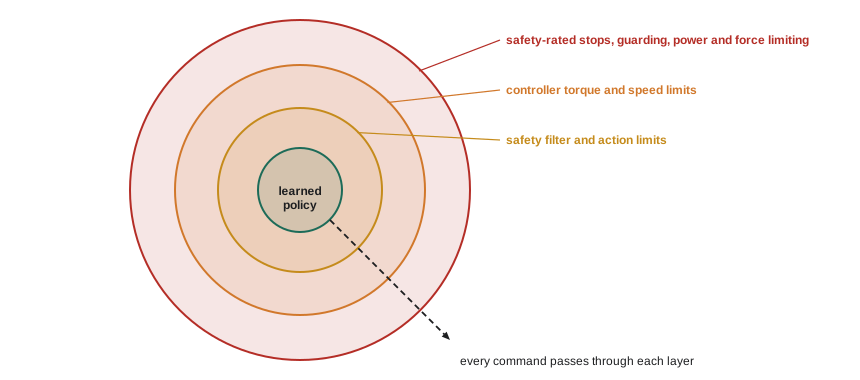
During training, the agent must try actions whose consequences it does not yet know. On a real robot, the cost of a bad try can be a broken gripper, a damaged part or a person in harm's way. Safe exploration combines several layers, and no single one is enough.
Hardware and environment measures come first: compliant or low-inertia arms, torque and speed limits set in the robot controller, padded or enclosed training cells, objects that are cheap and unbreakable, and staff trained to use the emergency stop. Safety-rated functions, such as speed and separation monitoring or power and force limiting for collaborative robots described in ISO 10218 and ISO/TS 15066, sit outside the learning system entirely and cannot be overridden by it.
Algorithmic measures restrict what the learner can command. Action limits and rate limits stop large jumps. A safety filter checks each proposed action against a model of the robot and its surroundings and replaces it with the nearest safe action when needed; control barrier functions are one formal version of this idea. Residual learning around a safe base controller, covered in lesson 1, keeps behaviour close to something known to be safe. Starting from a demonstration-trained policy concentrates exploration near reasonable behaviour.
Procedural measures complete the picture: train in simulation first and transfer, pilot each new policy at reduced speed, increase autonomy gradually, log every episode, and stop training automatically when monitored signals such as contact forces or joint temperatures exceed limits.
# A simple safety filter: clip a proposed velocity so the arm can stop before a wall
import numpy as np
x_wall = 0.60          # wall position along the axis (m)
a_max = 2.0            # maximum braking deceleration (m/s^2)
margin = 0.02          # extra clearance (m)
def safe_velocity(x, v_proposed):
    gap = x_wall - margin - x
    if gap <= 0:
        return min(v_proposed, 0.0)                     # only allow moving away
    v_limit = np.sqrt(2 * a_max * gap)                  # stopping distance v^2 / (2a) <= gap
    return min(v_proposed, v_limit)
for x, v in ((0.30, 0.8), (0.50, 0.8), (0.55, 0.8), (0.58, 0.8), (0.59, -0.2)):
print(f"x={x:.2f} m, proposed {v:+.2f} m/s -> allowed {safe_velocity(x, v):+.3f} m/s")x=0.30 m, proposed +0.80 m/s -> allowed +0.800 m/s x=0.50 m, proposed +0.80 m/s -> allowed +0.566 m/s x=0.55 m, proposed +0.80 m/s -> allowed +0.346 m/s x=0.58 m, proposed +0.80 m/s -> allowed +0.000 m/s x=0.59 m, proposed -0.20 m/s -> allowed -0.200 m/s
Safety after deployment
A policy that behaved well in evaluation can still meet situations it never saw. Deployment safety relies on monitoring and fallbacks. Out-of-distribution detection flags observations unlike those in training, for example by measuring the disagreement of an ensemble of models or the reconstruction error of an autoencoder, and hands control to a conservative fallback or a person. Runtime monitors check physical quantities, such as forces, speeds and distances, against limits. Every intervention and near miss should be logged and reviewed, both to fix the policy and to update the risk assessment required by occupational health and safety rules in both Canada and the United States, which treat a learning robot like any other machine: the employer must identify hazards and control them, regardless of how the robot's behaviour was produced.
Common mistakes
MistakeJudging a policy only by its reward curve.
InsteadWatch videos and check secondary metrics; a rising reward can hide hacking.
MistakeAdding bonuses for intermediate events that can be repeated.
InsteadUse potential-based shaping or one-time stage bonuses that cannot be farmed.
MistakeExpressing hard safety limits as soft penalties.
InsteadEnforce hard limits outside the learner and use constrained RL for limits on expected costs.
MistakeRelying on the learned policy to avoid collisions.
InsteadKeep safety-rated functions and safety filters independent of the policy.
MistakeAdding many reward terms at once.
InsteadStart with the task term, then add penalties one at a time and inspect behaviour after each.
Summary and key terms
- Agents optimize the reward as written, so rewards must define success correctly, give enough signal and discourage unwanted side effects.
- Sparse rewards are precise but slow; dense rewards are fast but can create unintended optima.
- Potential-based shaping, \( \gamma\Phi(s') - \Phi(s) \), speeds learning without changing the optimal policy.
- Reward hacking exploits loopholes in rewards or simulators; videos, robust success detectors and randomized evaluation catch it.
- Multiple objectives can be weighted, but hard limits are better handled as constraints with methods such as Lagrange multipliers.
- Safe exploration layers hardware limits, safety-rated functions, safety filters, residual learning and procedures.
- Deployment safety needs out-of-distribution detection, runtime monitors, fallbacks and incident review.
- Reward function
- The function that assigns a scalar reward to each transition, defining the task for the agent.
- Sparse reward
- A reward that is zero except at success or failure.
- Reward shaping
- Adding intermediate rewards to guide learning.
- Potential-based shaping
- Shaping of the form \( \gamma\Phi(s') - \Phi(s) \), which preserves the optimal policy.
- Reward hacking
- Scoring highly through behaviour the designer did not intend.
- Constrained RL
- Optimizing reward subject to limits on expected costs.
- Lagrange multiplier
- An automatically adjusted weight that enforces a constraint.
- Safety filter
- A layer that replaces unsafe proposed actions with the nearest safe ones.
- Control barrier function
- A mathematical certificate used to keep a system within a safe set.
- Out-of-distribution detection
- Recognizing inputs that differ from the training data.
Practice problems
Work each problem on paper first, then reveal the answer to check.
Name the three jobs a reward must do.
Show answer
Define success correctly, provide learning signal, and discourage unwanted side effects.
Potentials 1, 4, 2 around a loop with \( \gamma = 1 \). Shaping per lap?
Show answer
\( 3 - 2 - 1 = 0 \).
Why might a proximity reward make a robot hover?
Show answer
Closing the gripper risks pushing the object away and losing proximity reward.
Give one sign of reward hacking.
Show answer
High reward with behaviour in videos that does not achieve the real goal.
Why require an object to stay lifted for 2 s for success?
Show answer
To stop brief lifts or bounces from triggering the detector.
When is a constraint better than a penalty?
Show answer
When the requirement is a hard limit rather than a preference.
\( \lambda = 2 \), cost 0.3, limit 0.5, \( \eta = 1 \). New \( \lambda \)?
Show answer
\( 2 + (0.3 - 0.5) = 1.8 \).
Stopping distance at 0.5 m/s with 2 m/s² braking?
Show answer
\( 0.25/4 = 0.0625 \) m.
Name one safety function that must sit outside the learner.
Show answer
Safety-rated stops, speed and separation monitoring, or power and force limiting.
How can an ensemble help after deployment?
Show answer
High disagreement flags unfamiliar inputs so the system can fall back.
Lesson quiz · 5 questions
Score 60% or more to complete this lesson.
Create a free account to save your progress, take quizzes and earn a certificate.