Image filtering, edges and features

Most of an image is uninformative for geometry. A blank wall or a smooth floor gives no way to tell one pixel from its neighbour, so it cannot be matched between images or used to measure motion. What a robot can measure reliably are distinctive structures: edges where brightness changes sharply, and corners where edges meet. This lesson covers the operations that find them, starting with linear filtering, the workhorse of classical image processing, then gradients and edges, then corner detection and the descriptors that let a robot recognize the same corner in another image. These classical tools remain central in robotics because they are fast, well understood and precise to a fraction of a pixel, and learned features (lesson 9) are judged against them.

Linear filtering and convolution

A linear filter replaces each pixel by a weighted sum of its neighbours. The weights form a small array called a kernel, and sliding the kernel over the image is convolution, the same operation met in ROB-230 for one-dimensional signals:

The simplest kernel, a box filter, averages a 3 × 3 or 5 × 5 neighbourhood and reduces noise, but it blurs edges and creates ringing artefacts in the frequency domain. The Gaussian kernel, with weights \( h(x, y) \propto e^{-(x^2 + y^2)/2\sigma^2} \), is preferred: it smooths without ringing, its amount of smoothing is set by a single parameter σ, and it is separable, meaning a 2-D Gaussian blur equals a 1-D blur along rows followed by one along columns. Separability cuts the cost from \( k^2 \) to 2k multiplications per pixel for a k-wide kernel. A kernel about 6σ wide (rounded up to an odd number) captures more than 99 % of the weight.

Noise reduction by averaging follows the statistics of ROB-310: averaging n independent noisy pixels reduces the noise standard deviation by \( \sqrt{n} \). A 3 × 3 box filter averages nine pixels and cuts noise by a factor of three, at the cost of detail. Non-linear filters keep edges better. The median filter replaces a pixel with the median of its neighbourhood, which removes isolated salt-and-pepper noise such as dead pixels while leaving a step edge sharp, and the bilateral filter averages only neighbours of similar brightness.

Gradients and edges

An edge is a place where brightness changes quickly, so edges are found from the image gradient, the vector of partial derivatives \( (I_u, I_v) \). On a discrete image, derivatives are approximated by convolving with small difference kernels. The Sobel operator combines a difference in one direction with smoothing in the other:

The gradient magnitude \( \sqrt{I_u^2 + I_v^2} \) is large at edges, and the gradient direction \( \theta = \operatorname{atan2}(I_v, I_u) \) points across the edge, from dark to bright. Because differentiation amplifies noise (in frequency terms, it boosts high frequencies), images are almost always smoothed with a Gaussian first; the combined operation is a derivative-of-Gaussian filter.

The Canny edge detector, published in 1986 and still standard, turns gradient magnitudes into thin, connected edge curves in four steps: smooth with a Gaussian; compute gradient magnitude and direction; apply non-maximum suppression, keeping a pixel only if its magnitude is larger than its two neighbours along the gradient direction, which thins edges to one pixel; and apply hysteresis thresholding with two thresholds, keeping strong edge pixels and any weak ones connected to them. Hysteresis keeps edges continuous through slightly weaker sections while rejecting isolated noise. Robots use edges to find the boundaries of parts, lane markings, shelf fronts and doorways, and to fit lines and circles with the Hough transform or RANSAC (lesson 5).

Corners and the structure tensor

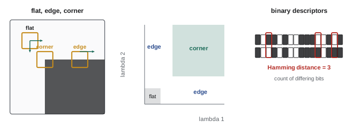
An edge locates position in only one direction: slide along an edge and the image looks the same. A corner, where the image changes in every direction, can be located in both coordinates, which makes corners ideal for matching and tracking. The Harris detector (Harris and Stephens, 1988) measures this by summing products of gradients over a small window W, giving the structure tensor

Its eigenvalues \( \lambda_1, \lambda_2 \) describe how the image changes as the window shifts. Both small: a flat region. One large and one small: an edge. Both large: a corner. Rather than computing eigenvalues, Harris used the response

with k around 0.04 to 0.06. R is large and positive at corners, negative at edges and small in flat regions. Shi and Tomasi (1994) showed that using \( \min(\lambda_1, \lambda_2) \) directly gives corners that track better; their 'good features to track' are the default in many visual odometry systems. Corner positions can be refined to around 0.1 pixel by fitting to the local gradient pattern.

import numpy as np

def conv2(img, k):
    """Same-size 2-D correlation with zero padding (enough for small kernels)."""
    kh, kw = k.shape
    p = np.pad(img, ((kh // 2,), (kw // 2,)))
    out = np.zeros_like(img, dtype=float)
    for i in range(kh):
        for j in range(kw):
            out += k[i, j] * p[i:i + img.shape[0], j:j + img.shape[1]]
    return out

# synthetic image: a bright square on a dark background
img = np.zeros((60, 60))
img[20:40, 20:40] = 100.0

sobel_u = np.array([[-1, 0, 1], [-2, 0, 2], [-1, 0, 1]], float)
Iu, Iv = conv2(img, sobel_u), conv2(img, sobel_u.T)

g = np.exp(-np.arange(-2, 3) ** 2 / 2.0)
G = np.outer(g, g); G /= G.sum()              # 5 x 5 Gaussian window, sigma 1
Suu, Svv, Suv = conv2(Iu * Iu, G), conv2(Iv * Iv, G), conv2(Iu * Iv, G)
R = Suu * Svv - Suv ** 2 - 0.05 * (Suu + Svv) ** 2

# local maxima above 10 % of the strongest response
thr = 0.1 * R.max()
peaks = []
for y in range(1, 59):
    for x in range(1, 59):
        if R[y, x] > thr and R[y, x] == R[y - 1:y + 2, x - 1:x + 2].max():
            peaks.append((x, y))
print("corners found:", peaks)
print("R at an edge midpoint (30, 20): %.0f" % R[20, 30])
print("R in a flat area (5, 5): %.0f" % R[5, 5])

corners found: [(20, 20), (39, 20), (20, 39), (39, 39)]
R at an edge midpoint (30, 20): -535523558
R in a flat area (5, 5): 0

Scale and the image pyramid

A corner detected with a 5 × 5 window in one image may look rounded and edge-like when the camera moves closer and the structure fills fifty pixels. To match features across changes of distance, detectors must work at several scales. The usual tool is an image pyramid: repeatedly blur and halve the image, and run the detector at each level. Scale-space theory formalizes this: blurring with Gaussians of increasing σ creates a family of images, and features are found where a response, such as the Laplacian of Gaussian or its approximation the difference of Gaussians, peaks in both position and scale. The scale at which a feature peaks tells how big it is, so the same physical structure is found at matching scales in near and far views.

Descriptors: SIFT, ORB and friends

Detecting a corner says where it is; matching it in another image needs a description of what it looks like. A descriptor is a vector computed from the image patch around a feature, designed so that the same physical point gives similar vectors in different images despite changes in viewpoint, lighting and scale.

• SIFT (scale-invariant feature transform, Lowe, 2004) finds difference-of-Gaussian peaks, assigns each a dominant orientation from local gradients, and describes a rotated, scaled patch by histograms of gradient directions in a 4 × 4 grid of cells with 8 orientation bins each, giving a 128-number vector. It is robust and accurate, and its patent expired in 2020, so it is now freely usable in OpenCV.
• ORB (oriented FAST and rotated BRIEF, Rublee and others, 2011) is built for speed. FAST finds corners by checking whether a ring of 16 pixels around a candidate has a long run of pixels all brighter or all darker than the centre. BRIEF describes the patch by 256 binary comparisons between pairs of pixels, rotated to the feature's orientation. Binary descriptors are compared with the Hamming distance, the number of differing bits, which modern processors compute in a single instruction. ORB-SLAM, one of the best-known visual SLAM systems, is built on ORB features.
• Others include SURF, AKAZE and BRISK, and learned descriptors such as SuperPoint (lesson 9), which often match better under large viewpoint and lighting changes.