
ROB-300 · Lesson 4 of 12 · 34 min
PID control of a robot joint
Most robot joints in the world are controlled by some form of PID: proportional, integral and derivative feedback on the joint position error. Industrial arms, collaborative robots, legged robots and drones all run PID or close relatives in their inner loops, often alongside the model-based terms of later lessons. PID is popular because it needs only a rough plant model, can be tuned on the machine, and in its derivative and integral terms already provides damping and the rejection of constant disturbances such as gravity. It also has well-known failure modes: integrator windup when the actuator saturates, noise amplification by the derivative, and limit cycles with friction. This lesson designs PID controllers for the joint model of lesson 3 by pole placement, compares this with classical tuning rules, and covers the practical details that turn a textbook PID into one that works on a robot.
The plant: independent joint control
Lesson 3 reduced each joint to an effective inertia J and viscous damping b driven by torque, with gravity, friction and coupling from other joints lumped into a disturbance torque d:
Controlling each joint separately with this simple model is called independent joint control. It works well when the gear ratio is high, because the disturbance is small compared with the motor torque and the inertia varies little. The controller sees a position error \( e = q_d - q \) and computes a torque. The plant has a pole at the origin, a pure integrator from speed to position, and a pole at \( -b/J \). Our job is to place the closed-loop poles where we want them.
Proportional control
With \( \tau = K_pe \), the closed loop from desired to actual position is
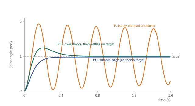
a second-order system with \( \omega_n = \sqrt{K_p/J} \) and \( \zeta = b/(2\sqrt{K_pJ}) \). Raising \( K_p \) speeds the response but lowers the damping, and since b is usually small, a fast P controller oscillates badly. Its other weakness appears with a constant disturbance such as gravity: at steady state \( K_pe_{ss} = d \), so the joint sags by \( e_{ss} = d/K_p \).
Worked problem
Gravity sag under proportional control
A joint with J = 1.5 kg·m² and b = 0.5 N·m·s/rad must hold a link whose gravity torque is 13.7 N·m. With \( K_p \) = 600 N·m/rad, find the steady sag, the natural frequency and the damping ratio.
Show solution
- Sag: \( e_{ss} = 13.7/600 = 0.0228 \) rad, about 1.3°.
- Natural frequency: \( \omega_n = \sqrt{600/1.5} = 20 \) rad/s.
- Damping: \( \zeta = 0.5/(2\sqrt{600 \times 1.5}) = 0.5/60 = 0.0083 \).
Answer: The arm sags 1.3°, and with ζ ≈ 0.008 any disturbance would set it ringing at about 3.2 Hz for many seconds. Proportional control alone is unusable here: it needs damping, which derivative action supplies, and zero steady error, which integral action supplies.
PD control and pole placement
Adding derivative action, \( \tau = K_pe + K_d\dot{e} \), and taking \( \dot{q}_d = 0 \) for a set-point, gives the characteristic polynomial
Now the two closed-loop poles can be placed independently: \( K_p \) sets the natural frequency and \( K_d \) sets the damping. A common choice for robot joints is critical damping, ζ = 1, the fastest response without overshoot, because overshoot means the robot moves past its target and may hit something. The gains follow directly:
Physically, a PD controller is a virtual spring and damper connecting the joint to its target. The derivative should be taken of the measured position, \( -K_d\dot{q} \), rather than of the error when the set-point jumps, to avoid a huge torque spike at each step change (derivative kick). PD control still sags under gravity by \( d/K_p \), but with damping the gain can be raised until the sag is acceptably small.
Worked problem
PD gains by pole placement
For the joint of the previous example, choose PD gains for \( \omega_n \) = 20 rad/s and critical damping. What is the steady gravity sag?
Show solution
- \( K_p = J\omega_n^2 = 1.5 \times 400 = 600 \) N·m/rad.
- \( K_d = 2 \times 1 \times 20 \times 1.5 - 0.5 = 59.5 \) N·m·s/rad.
- Sag is unchanged at \( 13.7/600 = 0.0228 \) rad.
Answer: \( K_p = 600 \) and \( K_d = 59.5 \). The step response now rises without overshoot and settles in about \( 4.75/\omega_n \approx 0.24 \) s, but the arm still sags 1.3° unless gravity is compensated (lesson 9) or integral action is added.
PID control
Integral action accumulates the error so that any steady error causes a steadily growing torque until the error is gone:
The closed loop is now third order. By the final value theorem of ROB-230, a constant disturbance produces zero steady error, because the integrator places a zero at s = 0 in the transfer function from disturbance to error. A convenient pole-placement choice is a triple pole at \( s = -\omega \), which gives a critically damped, overshoot-free disturbance response. Matching \( J(s + \omega)^3 = Js^3 + 3J\omega s^2 + 3J\omega^2s + J\omega^3 \) term by term:
Other placements trade speed against overshoot; the Routh–Hurwitz test of lesson 5 shows that stability requires \( (b + K_d)K_p > JK_i \), so too much integral gain destabilizes the loop.
Worked problem
PID gains for a triple pole
Design a PID for the same joint with a triple closed-loop pole at −15 rad/s. Check the Routh–Hurwitz condition.
Show solution
- \( K_d = 3 \times 1.5 \times 15 - 0.5 = 67.0 \) N·m·s/rad.
- \( K_p = 3 \times 1.5 \times 225 = 1012.5 \) N·m/rad.
- \( K_i = 1.5 \times 3375 = 5062.5 \) N·m/(rad·s).
- Check: \( (b + K_d)K_p = 67.5 \times 1012.5 = 68{,}344 > JK_i = 7{,}594 \). Stable.
Answer: \( K_p \approx 1013 \), \( K_i \approx 5063 \), \( K_d = 67 \). Gravity sag is eliminated, with the error decaying as \( (1 + \omega t + \omega^2t^2/2)e^{-\omega t} \)-shaped transients that die out within about 0.5 s. A step in the set-point overshoots somewhat, because the PI zeros speed up the reference response; a set-point filter or applying \( K_p \) to the measurement can remove it.
Classical tuning rules
When a model is not available, PID gains can be found by experiment. The Ziegler–Nichols ultimate-gain method, published in 1942, is the best known: with integral and derivative action off, raise the proportional gain until the loop oscillates steadily; record that ultimate gain \( K_u \) and the oscillation period \( T_u \); then set
| Controller | \( K_p \) | \( T_i \) (integral time) | \( T_d \) (derivative time) |
|---|---|---|---|
| P | \( 0.5K_u \) | — | — |
| PI | \( 0.45K_u \) | \( T_u/1.2 \) | — |
| PID | \( 0.6K_u \) | \( T_u/2 \) | \( T_u/8 \) |
These settings give fast but oscillatory responses, about a quarter-amplitude decay per cycle, which is usually too aggressive for robots. They are a starting point to be softened. Driving a robot joint into sustained oscillation is also risky, so relay auto-tuning, which induces a small controlled oscillation with an on–off torque, or model-based tuning from a measured step response, is safer in practice. For a pure double-integrator joint with little damping, P control is already marginally stable, so the ultimate-gain experiment does not apply directly; it suits joints with an extra lag such as a filter or delay.
Worked problem
Ziegler–Nichols settings
A belt-driven joint oscillates steadily when \( K_p \) reaches 80 N·m/rad, with period 0.25 s. Find Ziegler–Nichols PID gains.
Show solution
- \( K_p = 0.6 \times 80 = 48 \) N·m/rad.
- \( T_i = 0.25/2 = 0.125 \) s, so \( K_i = 48/0.125 = 384 \) N·m/(rad·s).
- \( T_d = 0.25/8 = 0.03125 \) s, so \( K_d = 48 \times 0.03125 = 1.5 \) N·m·s/rad.
Answer: \( K_p = 48 \), \( K_i = 384 \), \( K_d = 1.5 \). Expect noticeable overshoot; reducing \( K_p \) by a third and doubling \( T_i \) is a common softening for motion systems.
Saturation and integrator windup
Every actuator has a torque limit. When a large step command saturates the motor, the error stays large for longer than the linear design assumed, and the integrator keeps accumulating it. When the joint finally reaches the target, the integrator holds a large stored value that drives the joint well past the target, producing a big overshoot and slow recovery. This is integrator windup. Two standard fixes are:
- Clamping (conditional integration): stop integrating while the output is saturated and the error would push it further into saturation.
- Back-calculation: feed the difference between the saturated and unsaturated commands back into the integrator through a gain \( 1/T_t \), bleeding off the excess. A tracking time \( T_t \) between \( T_d \) and \( T_i \) is a common choice.
Robot controllers also clamp the integrator to a maximum torque contribution and often reset or freeze it during large motions, enabling it only near the target where its job, removing small steady errors, is done. With static friction, an integrator can still cause the stick-slip limit cycle of lesson 3; remedies include friction feedforward, a small dead zone on the integrator, or integral action only on the velocity loop.
import numpy as np
J, b, tmax = 1.5, 0.5, 40.0                 # joint, torque limit 40 N m
Kp, Ki, Kd = 1012.5, 5062.5, 67.0
def run(antiwindup, T=1.5, h=1e-4):
    q = qd = integ = 0.0; peak = 0.0; target = 1.0
    for k in range(int(T/h)):
        e = target - q
        u = Kp*e + Ki*integ - Kd*qd
        tau = np.clip(u, -tmax, tmax)
        if antiwindup:
            integ += h*(e + (tau - u)/(Ki*0.05))      # back-calculation, Tt = 0.05 s
        else:
            integ += h*e
        qdd = (tau - b*qd)/J
        q += h*qd; qd += h*qdd
        peak = max(peak, q)
    return peak, q
for aw in (False, True):
    peak, qend = run(aw)
print(f"anti-windup={aw!s:5}: overshoot {max(0.0, 100*(peak-1)):6.1f} %, q(1.5 s) = {qend:.3f} rad")anti-windup=False: overshoot 152.6 %, q(1.5 s) = -2.686 rad anti-windup=True : overshoot 0.0 %, q(1.5 s) = 1.000 rad
Without anti-windup the saturated step overshoots by more than 150 % and is still swinging wildly 1.5 s later, because the integrator stores the error accumulated during the long saturated climb and the saturated loop cannot unload it quickly; with back-calculation the joint arrives without overshoot and settles cleanly on the target. The torque limit makes this step far slower than the linear design predicted, a reminder that trajectory planning (lesson 8) should keep commands within the actuator's capability in the first place.
Practical PID details
Several further details separate a working joint controller from a textbook one:
- Derivative filtering: the derivative of a quantized encoder signal is noisy (ROB-230). Use a filtered velocity, for example a first-order low-pass with a cutoff a few times the loop bandwidth, or a velocity estimate from an observer (lesson 6).
- Velocity feedforward: when following a moving target, add \( K_d\dot{q}_d \) or better a model-based feedforward, so that the controller does not rely on error to generate the torque needed for motion.
- Gain scheduling: when inertia varies with configuration or payload, scale the gains with the estimated inertia, \( K_p = \hat{J}(\mathbf{q})\omega_n^2 \), so the loop keeps its intended speed and damping.
- Sample rate: a digital PID should run at least 10 to 20 times faster than the closed-loop bandwidth; lesson 11 covers discretization and delay.
- Bumpless transfer: when switching from manual to automatic mode or between gain sets, initialize the integrator so the commanded torque does not jump.
Worked problem
Gain scheduling with payload
A joint tuned with \( K_p \) = 600 N·m/rad for J = 1.5 kg·m² picks up a payload that raises J to 2.4 kg·m². With fixed gains, what happen to \( \omega_n \) and ζ (with \( K_d \) = 59.5, b = 0.5)? What gains restore the design?
Show solution
- Fixed gains: \( \omega_n = \sqrt{600/2.4} = 15.8 \) rad/s; \( \zeta = 60/(2\sqrt{600 \times 2.4}) = 60/75.9 = 0.79 \).
- Restored gains: \( K_p = 2.4 \times 400 = 960 \); \( K_d = 2 \times 20 \times 2.4 - 0.5 = 95.5 \).
Answer: With fixed gains the joint slows to 15.8 rad/s and becomes slightly underdamped (ζ ≈ 0.79, about 2 % overshoot). Scaling the gains with the new inertia to \( K_p \) = 960 and \( K_d \) = 95.5 restores 20 rad/s and critical damping.
Common mistakes
MistakeTaking the derivative of the error when the set-point steps
InsteadDifferentiate the measurement, \( -K_d\dot{q} \), to avoid derivative kick.
MistakeLetting the integrator run while the motor is saturated
InsteadUse clamping or back-calculation anti-windup.
MistakeUsing Ziegler–Nichols settings unchanged on a robot
InsteadThey are deliberately aggressive; soften them and verify overshoot.
MistakeRaising integral gain to remove error faster without checking stability
InsteadToo much \( K_i \) violates \( (b + K_d)K_p > JK_i \) and destabilizes the loop.
MistakeKeeping fixed gains when payload changes a lot
InsteadSchedule gains with estimated inertia or use model-based control.
Summary and key terms
- Independent joint control treats each joint as \( 1/(s(Js + b)) \) with gravity, friction and coupling as disturbances.
- P control alone is poorly damped and sags under gravity by \( d/K_p \).
- PD control places both poles: \( K_p = J\omega_n^2 \), \( K_d = 2\zeta\omega_nJ - b \); it is a virtual spring and damper.
- PID removes steady error from constant disturbances; a triple pole at −ω gives \( K_p = 3J\omega^2 \), \( K_i = J\omega^3 \), \( K_d = 3J\omega - b \).
- Ziegler–Nichols rules give aggressive starting gains from an ultimate gain and period.
- Actuator saturation causes integrator windup; clamping or back-calculation prevents it.
- Practical PID needs filtered derivatives, feedforward, gain scheduling, adequate sample rates and bumpless transfer.
- Independent joint control
- Controlling each joint with its own loop, treating coupling as disturbance.
- Proportional gain
- The gain \( K_p \) multiplying position error; a virtual spring.
- Derivative gain
- The gain \( K_d \) on velocity error; a virtual damper.
- Integral gain
- The gain \( K_i \) on accumulated error, which removes steady error.
- Critical damping
- Damping ratio 1, the fastest response without overshoot.
- Derivative kick
- A torque spike caused by differentiating a stepped error.
- Ultimate gain
- The proportional gain at which the loop oscillates steadily.
- Integrator windup
- Excess integral accumulation during saturation that causes overshoot.
- Back-calculation
- An anti-windup scheme feeding the saturation excess back to the integrator.
- Gain scheduling
- Changing controller gains with operating conditions such as inertia.
Practice problems
Work each problem on paper first, then reveal the answer to check.
A joint has J = 0.5 kg·m². What \( K_p \) gives \( \omega_n \) = 30 rad/s with PD control?
Show answer
450 N·m/rad.
With b = 0.2, what \( K_d \) gives ζ = 1 for that joint?
Show answer
\( 2 \times 30 \times 0.5 - 0.2 = 29.8 \).
Gravity torque 5 N·m and \( K_p \) = 250 N·m/rad. Find the PD sag.
Show answer
0.02 rad.
Give PID gains for a triple pole at −10 with J = 1 and b = 0.
Show answer
\( K_d = 30 \), \( K_p = 300 \), \( K_i = 1000 \).
Is \( s^3 + 4s^2 + 5s + 30 \) stable?
Show answer
No; \( 4 \times 5 = 20 < 30 \).
Ziegler–Nichols: \( K_u \) = 50, \( T_u \) = 0.4 s. Give PI gains.
Show answer
\( K_p = 22.5 \), \( T_i = 0.333 \) s, \( K_i = 67.5 \).
Why does a PD controller act like a spring and damper?
Show answer
Torque is proportional to displacement from the target and to velocity.
What causes integrator windup?
Show answer
Integrating error while the actuator is saturated.
At what rate should a PID run for a 10 Hz closed-loop bandwidth?
Show answer
At least 100 to 200 Hz, preferably more.
Why differentiate the measurement rather than the error?
Show answer
To avoid a torque spike when the set-point changes suddenly.
Lesson quiz · 5 questions
Score 60% or more to complete this lesson.
Create a free account to save your progress, take quizzes and earn a certificate.