Force control: impedance, admittance and hybrid control

Everything so far has controlled motion in free space. Many of the most valuable robot tasks involve contact: inserting a peg, polishing a surface, assembling parts, opening a door, handing an object to a person, or a legged robot's foot striking the ground. In contact, pure position control is a poor idea. A stiff position controller pressed against a rigid surface with even a millimetre of position error generates enormous forces, and a small error in the modelled location of a part can break the part or the robot. Force control regulates the interaction itself: the force exerted, or the relationship between force and motion. This lesson covers the contact model, direct force control, impedance and admittance control, which shape the robot's apparent mechanical behaviour, hybrid position/force control, and the stability problems peculiar to contact.

Contact as a spring

The simplest model of a contacted environment is a spring of stiffness \( k_e \) located at position \( x_e \): when the tool penetrates by \( x - x_e > 0 \), the environment pushes back with force \( F = k_e(x - x_e) \). Real stiffnesses span a vast range: a sponge might be 100 N/m, a human hand 1,000 to 5,000 N/m, wood or a plastic part around \( 10^5 \) N/m, steel in contact effectively \( 10^6 \) N/m or more once the robot's own structure is included. The ratio of the robot's controlled stiffness to the environment's stiffness largely decides who 'wins' in contact: a soft controller against a hard environment controls force well and position poorly; a stiff controller against a soft environment controls position well and force poorly.

Mapping forces to joint torques

Forces at the tool relate to joint torques through the transpose of the manipulator Jacobian (ROB-210): a wrench \( \mathbf{F} \) at the end effector requires joint torques

This follows from virtual work: the power at the joints, \( \boldsymbol{\tau}^{\mathsf{T}}\dot{\mathbf{q}} \), must equal the power at the tool, \( \mathbf{F}^{\mathsf{T}}\dot{\mathbf{x}} = \mathbf{F}^{\mathsf{T}}\mathbf{J}\dot{\mathbf{q}} \). The relation lets a torque-controlled robot apply a chosen force without any force sensor, provided friction and the dynamic model are well known, and lets a force sensor reading be expressed as joint torques. Near singularities, \( \mathbf{J}^{\mathsf{T}} \) maps large tool forces to small joint torques in some directions, which is why a nearly straight arm can resist huge forces along its length.

Direct force control

When the task is to hold a specified contact force, for example pressing a polishing tool with 15 N, the simplest approach measures the force with a wrist force/torque sensor and closes a loop on the force error. Because the contact force is proportional to penetration, a force loop through a position-controlled robot is effectively a loop on position with gain \( k_e \): stiff environments make the loop gain high and threaten stability, soft environments make it sluggish. Integral action is usually included to remove steady force error, and the force signal is filtered because force sensors are noisy. Direct force control works when the robot is always in contact; it behaves badly during the transition from free space to contact, when there is no force to feed back and the robot accelerates toward the surface until it hits.

Impedance control

Impedance control, formulated by Neville Hogan in 1985, takes a different view: rather than controlling force or position, control the dynamic relationship between them. The robot is made to behave like a chosen mass-spring-damper system attached to a reference trajectory \( \mathbf{x}_r \):

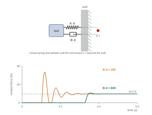
In free space, with no external force, the robot follows the reference like a position controller. In contact, it yields like a spring, and the force it exerts is set by the stiffness and the penetration of the reference into the surface. The same controller handles both phases and the transition between them, which is its great advantage. A simple implementation on a torque-controlled robot, with the desired inertia left as the robot's own and gravity compensated, is

a Cartesian PD law mapped to joint torques. This is how collaborative arms with joint torque sensing provide their compliant, safe behaviour: a person pushing the arm feels a spring and damper, not a rigid machine. Stiffness and damping can be set separately for each direction, for example stiff in the plane of a surface and compliant normal to it.

Admittance control

Impedance control needs a robot whose joint torques can be commanded accurately: direct-drive, low-ratio or torque-sensed joints. Most industrial robots have stiff position controllers behind high-ratio gearboxes and do not accept torque commands. For them, admittance control inverts the causality. A force/torque sensor measures the contact force, a virtual dynamic model computes the motion that a mass-spring-damper would make in response, and that motion is sent to the robot's position controller:

where \( \mathbf{x}_c \) is the commanded position, integrated in software at each control step. Impedance and admittance control are complementary. Impedance control renders soft behaviour well but struggles to render high stiffness, because the robot's own friction and limited torque bandwidth get in the way. Admittance control renders stiff behaviour well, since the inner position loop is stiff, but is prone to instability when rendering low inertia and damping against stiff environments: the force loop gain becomes too high. Hand-guiding of industrial robots through a wrist force sensor, a common way to teach positions, uses admittance control with low virtual mass and damping in free space.

Hybrid position/force control

Many tasks need position control in some directions and force control in others at the same time. Wiping a table requires pressing down with a controlled force while moving across the surface along a position trajectory. Raibert and Craig's hybrid position/force control, from 1981, splits task space with a diagonal selection matrix S, with ones in the force-controlled directions and zeros in the position-controlled ones:

Here \( \mathbf{F}_{\text{force}} \) comes from a force loop and \( \mathbf{F}_{\text{position}} \) from a position loop, both expressed in a task frame aligned with the contact, for example with z normal to the surface. The choice follows the natural constraints of the task: where the environment prevents motion, control force; where it prevents force (free directions), control position. A peg-in-hole insertion controls force along the hole axis and lateral position, while allowing small lateral compliance so the peg can centre itself. A known difficulty is that the selection must match the actual contact geometry; if the surface is tilted relative to the assumed task frame, the force and position loops fight each other.

Contact stability and passivity

Contact makes control harder for three reasons. First, the environment stiffness multiplies the loop gain, as in direct force control, so a loop tuned in free space can go unstable against a hard surface. Second, the instant of impact is a discontinuity: the robot arrives with momentum, and a stiff, poorly damped controller bounces, repeatedly losing and regaining contact, a behaviour called chatter. Third, sampling, delay and sensor filtering, all harmless in free space, can turn a nominally stable contact unstable because the stiff contact has a high natural frequency, \( \omega_c = \sqrt{(K_d + k_e)/m} \), possibly above the controller's ability to respond.

A powerful design principle is passivity: if the controlled robot, seen from its contact point, never generates net energy, it will remain stable when coupled to any passive environment, whether soft, hard, or a human. Impedance controllers with positive stiffness and damping are passive in continuous time; digital implementation adds energy through sampling, which limits the stiffness that can be rendered stably for a given sample rate and damping. A widely cited guideline from haptics, the work of Colgate and colleagues in the 1990s, states that a virtual wall of stiffness K rendered with sample time T and damping B, on a device with physical damping b, is passive when \( b > KT/2 + B \), where B here is the virtual damping in the discrete implementation. Ordinary engineering practice is to add damping, lower stiffness near contact, approach surfaces slowly, and filter force signals with care.

import numpy as np
m, Kd, ke, xe = 4.0, 2000.0, 5.0e4, 0.0            # tool mass, impedance stiffness, wall at x = 0
def contact(Bd, h=1e-5, T=0.6):
    x, v, xr = -0.02, 0.0, 0.010                   # start 20 mm before wall, reference 10 mm into it
    Fpeak = 0.0; bounces = 0; incontact = False
    for k in range(int(T/h)):
        Fe = ke*(x - xe) if x > xe else 0.0         # wall force on tool, pushing back
        if (x > xe) and not incontact: bounces += 1
        incontact = x > xe
        F = Kd*(xr - x) - Bd*v - Fe
        v += h*F/m; x += h*v
        Fpeak = max(Fpeak, Fe)
    return Fpeak, Fe, bounces
for Bd in (20.0, 180.0, 600.0):
    Fpk, Fend, nb = contact(Bd)
    print(f"Bd = {Bd:5.0f} N s/m: peak force {Fpk:6.1f} N, final {Fend:5.1f} N, contacts made {nb}")

Bd =    20 N s/m: peak force  256.9 N, final   0.0 N, contacts made 5
Bd =   180 N s/m: peak force   66.9 N, final  19.2 N, contacts made 2
Bd =   600 N s/m: peak force   21.3 N, final  19.2 N, contacts made 1

With light damping the tool strikes the wall at over 250 N, bounces off and is still chattering against it after 0.6 s; with moderate damping the peak falls to about 67 N and the tool bounces once before settling at 19.2 N; with heavy damping the approach is slow and the force rises almost without overshoot to the 19.2 N predicted by the series-spring calculation. Approach speed and damping, more than stiffness, decide the impact force.