
ROB-110 · Lesson 3 of 12 · 30 min
Python for robot programs
Python is the language most people use to write their first robot programs, and many professional robots use it for high-level behaviour, testing and tools. It is quick to write, easy to read, and has excellent libraries for numerical work, vision and machine learning. ROS 2 supports it through a client library called rclpy, alongside rclcpp for C++. This lesson builds on the Python you learned in CMPUT-174 and focuses on the habits that matter when code controls a physical machine: organizing state in classes, working with arrays of sensor data in NumPy, keeping time correctly in loops, and making sure that errors stop a robot safely rather than leaving it running blind.
Python or C++?
Robot software is a mix of languages. Low-level drivers and fast control loops are usually written in C or C++ because they compile to efficient machine code with predictable timing. Python is interpreted, slower and has occasional pauses for memory management, so it is a poor choice for a loop that must run every millisecond. But a great deal of robot software runs at 10 to 100 Hz, spends most of its time waiting for messages, or calls libraries such as NumPy and OpenCV that are themselves written in C. For that code Python's speed of development wins. In ROS 2, Python and C++ nodes communicate seamlessly, so teams commonly prototype in Python and rewrite only the parts that profiling shows to be too slow.
| Task | Typical rate | Common language |
|---|---|---|
| Motor current or torque loop | 1 to 20 kHz | C on a microcontroller |
| Joint position control | 100 Hz to 1 kHz | C++ |
| Mobile base velocity commands | 10 to 50 Hz | C++ or Python |
| Mission logic and state machines | 1 to 10 Hz | Python |
| Data analysis, tests and tools | Not time-critical | Python |
Organizing robot state with classes
A robot program has to remember things: its estimated position, the latest sensor readings, the current goal, the settings it was started with. Scattering these across global variables quickly becomes unmanageable. Classes group related data and the functions that act on it, and ROS 2 nodes in Python are themselves classes, as you will see in lesson 6. A dataclass is a compact way to define a class that mainly holds data: Python writes the constructor and a readable printed form for you.
The listing below models a differential-drive robot, the two-wheeled base you met in ROB-100. A Pose2D dataclass holds the position and heading, and a DiffDriveModel class updates the pose from a forward speed v and a turning rate ω over a short time step, using the same geometry as wheel odometry. The program drives the model forward, turns it left on the spot and drives it forward again.
import math
from dataclasses import dataclass


@dataclass
class Pose2D:
    x: float = 0.0
    y: float = 0.0
    theta: float = 0.0  # heading in radians


class DiffDriveModel:
    """Tracks the pose of a differential-drive robot."""

    def __init__(self, wheel_base):
        self.wheel_base = wheel_base
        self.pose = Pose2D()

    def update(self, v, w, dt):
        """Advance the pose for dt seconds at speed v and turn rate w."""
        p = self.pose
        p.x += v * math.cos(p.theta) * dt
        p.y += v * math.sin(p.theta) * dt
        p.theta += w * dt


robot = DiffDriveModel(wheel_base=0.3)
for step in range(20):          # 2 s straight at 0.5 m/s
    robot.update(0.5, 0.0, 0.1)
for step in range(10):          # 1 s turning left at 90 deg/s
    robot.update(0.0, math.pi / 2, 0.1)
for step in range(20):          # 2 s straight again
    robot.update(0.5, 0.0, 0.1)
p = robot.pose
print(f"x = {p.x:.2f} m, y = {p.y:.2f} m, "
f"heading = {math.degrees(p.theta):.0f} deg")x = 1.00 m, y = 1.00 m, heading = 90 deg
The robot ends one metre forward and one metre to the left, facing 90 degrees, as you would expect from the commands. Small design choices make this code easier to reuse: the wheel base is passed to the constructor rather than hard-coded, the time step is an argument so the same class works at any loop rate, and the angle is kept in radians, the unit every maths library expects. Type hints, docstrings and names that say what a value means, such as wheel_base rather than wb, cost little and save a great deal of confusion when a teammate reads your node at midnight before a competition.
The update uses simple Euler integration: it assumes the heading stays constant during each step. That is accurate when the step is small compared with how fast the robot turns. Halving the time step roughly halves the error, so a model updated at 50 Hz tracks a turning robot better than one updated at 5 Hz. You will meet better integration methods and the full odometry equations in ROB-210, but the habit of asking how a time step affects accuracy starts here.
Working with sensor data in NumPy
Sensors produce arrays of numbers: a laser scanner returns hundreds of distances per scan, a depth camera hundreds of thousands per frame. Processing them with Python loops is slow; NumPy processes whole arrays at once in compiled code, often a hundred times faster, and the code is shorter. The key ideas are that arithmetic on arrays applies element by element, that comparisons produce arrays of true and false values called masks, and that a mask can select elements from another array.
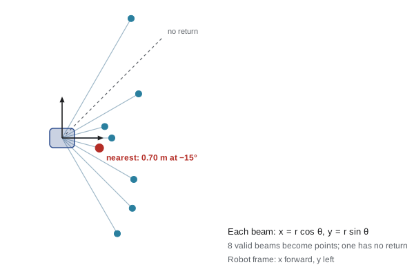
A two-dimensional laser scan reports each beam's range r at a known angle θ. Converting to Cartesian coordinates in the sensor's frame uses the familiar polar-to-Cartesian formulas, applied to all beams at once:
Scanners report beams that hit nothing as infinity or as a value outside their valid range, so real code removes them first. The listing builds a small simulated scan, removes the invalid beam with a mask, converts the rest to points and finds the nearest obstacle.
import numpy as np

# a simulated laser scan: 9 beams from -60 to +60 degrees
angles = np.radians(np.linspace(-60, 60, 9))
ranges = np.array([2.0, 1.8, 1.5, 0.7, 0.9, 0.8, 1.6, np.inf, 2.5])

valid = np.isfinite(ranges)          # drop beams with no return
x = ranges[valid] * np.cos(angles[valid])
y = ranges[valid] * np.sin(angles[valid])

j = np.argmin(ranges[valid])         # nearest valid beam
print("points:", valid.sum())
print(f"nearest: {ranges[valid][j]:.2f} m at "
      f"{np.degrees(angles[valid][j]):+.0f} deg")
print(f"as a point: x = {x[j]:.2f} m, y = {y[j]:.2f} m")points: 8 nearest: 0.70 m at -15 deg as a point: x = 0.68 m, y = -0.18 m
Worked problem
Checking one point by hand
The nearest beam in the listing has range 0.70 m at an angle of −15°. Verify the printed x and y values.
Show solution
- \( \cos(-15^\circ) \approx 0.966 \) and \( \sin(-15^\circ) \approx -0.259 \).
- \( x = 0.70 \times 0.966 \approx 0.68 \) m.
- \( y = 0.70 \times (-0.259) \approx -0.18 \) m.
- A negative y means the obstacle is to the robot's right, since y points left in the usual robot convention.
Answer: x ≈ 0.68 m and y ≈ −0.18 m, matching the program. The obstacle is ahead and slightly to the right.
Note that NumPy's argmin was applied to the filtered array, not the original, so the index j matches the x and y arrays. Keeping track of which array an index refers to after filtering is one of the most common sources of subtle bugs in sensor code. Another is mixing degrees and radians: NumPy's trigonometric functions expect radians, so convert once, at the edge of your program, and work in radians everywhere else.
Keeping time in loops
Robot programs run in loops: read sensors, decide, command actuators, wait, repeat. The loop must run at a steady rate, because controllers and estimators assume a known time step. Two time functions matter. time.time() returns the wall-clock time, which can jump when the clock is synchronized or changed; time.monotonic() never goes backwards and is the right choice for measuring intervals. In ROS 2 you will normally let the framework call your code from a timer, but understanding what goes wrong with hand-written loops explains why.
The naive approach is to do the work and then call time.sleep for the full period. But the work itself takes time, so each iteration lasts the work time plus the sleep, and the loop runs slower than intended. The fix is to schedule against deadlines: keep track of when the next iteration should start and sleep only until then. The listing simulates both approaches for a 50 Hz loop whose work takes 12 milliseconds, without actually sleeping, so the result is exact.
# Simulated timing: each loop does 12 ms of work, then waits.
period = 0.020                 # target 50 Hz
work = 0.012

# naive: work, then sleep a full period every time
t = 0.0
for k in range(500):
    t += work + period
print(f"naive: 500 loops took {t:.2f} s, "
      f"rate {500 / t:.1f} Hz")

# deadline-based: sleep only until the next tick
t, next_tick = 0.0, 0.0
for k in range(500):
    t += work
    next_tick += period
    t = max(t, next_tick)      # sleep until the deadline
print(f"deadline: 500 loops took {t:.2f} s, "
f"rate {500 / t:.1f} Hz, busy {work / period:.0%}")naive: 500 loops took 16.00 s, rate 31.2 Hz deadline: 500 loops took 10.00 s, rate 50.0 Hz, busy 60%
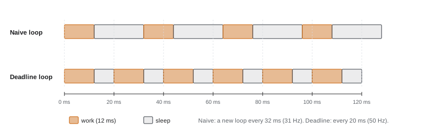
The naive loop runs at about 31 Hz instead of 50 Hz, a 38 per cent error that would make a controller tuned for 50 Hz behave quite differently. The deadline-based loop holds 50 Hz and spends 60 per cent of each period working. That fraction, the utilization, is worth computing for every loop: if the work ever takes longer than the period, the loop cannot keep up, and you must make the work faster, lower the rate or move it to another thread or process. Real loops also show jitter, small random variations in when each iteration starts, caused by the operating system scheduling other processes; lesson 6 shows how to measure it in ROS 2.
Worked problem
Utilization and headroom
A node must process each laser scan before the next arrives. The scanner runs at 15 Hz and processing takes 48 ms on average, with occasional scans taking 70 ms. Is the node fast enough?
Show solution
- Period: \( 1/15 \approx 66.7 \) ms.
- Average utilization: \( 48 / 66.7 \approx 72\% \), which leaves some headroom on average.
- The 70 ms worst case exceeds the 66.7 ms period, so occasionally a scan will arrive before the previous one is finished.
- With a queue depth of 1, the node simply drops the stale scan and processes the newest one; with a deep queue it falls further and further behind.
Answer: On average yes, but not in the worst case. Keep only the latest scan, optimize the slow path, or reduce the work so the worst case fits within 66.7 ms.
Failing safely
When a program that controls a robot crashes, the robot does not politely stop. A motor controller that received a velocity command will usually keep executing it until it receives another command or until its own watchdog timer expires. Software therefore needs to handle errors deliberately. Python's try and finally statements guarantee that cleanup code runs whether the protected block finishes normally, raises an exception or is interrupted by Ctrl+C. Put the code that stops actuators in a finally block, or in the shutdown handler that ROS 2 provides, so that every exit path leaves the robot in a safe state.
class FakeMotor:
    def __init__(self):
        self.speed = 0.0

    def set_speed(self, s):
        self.speed = s
        print(f"motor speed set to {s}")


def drive(motor, readings):
    try:
        for r in readings:
            if r < 0:
                raise ValueError(f"bad sensor reading {r}")
            motor.set_speed(min(r, 1.0))
    finally:
        motor.set_speed(0.0)   # always runs, even after an error


m = FakeMotor()
try:
    drive(m, [0.4, 0.8, -1.0, 0.6])
except ValueError as err:
    print("stopped because:", err)
print("final speed:", m.speed)motor speed set to 0.4 motor speed set to 0.8 motor speed set to 0.0 stopped because: bad sensor reading -1.0 final speed: 0.0
The third sensor reading is invalid, so drive raises an exception, but the finally block still sets the speed to zero before the error reaches the caller. Software stops are not the only safety layer: real robots also have hardware emergency stops, controller watchdogs that stop the motors if commands cease, and limits enforced in firmware. ROB-450 covers these in depth. But good software should never be the reason a robot keeps moving after something has gone wrong.
Writing code others can maintain
Robot software is usually written by teams and lives for years. A few habits pay off quickly. Follow the PEP 8 style guide so that your code looks like everyone else's; tools such as flake8 or ruff check it automatically, and ROS 2's own build tests can run them. Use the logging facilities rather than print, so that messages have severity levels and timestamps and can be filtered; in ROS 2 that means the node's logger. Keep hardware access, algorithms and ROS plumbing in separate functions or classes so that you can test the algorithm with fake data on a laptop, as the DiffDriveModel above can be tested without a robot. And write small automated tests with pytest for anything with arithmetic in it, because a sign error in a heading calculation is much cheaper to find in a test than in a robot driving into a wall.
Common mistakes
MistakeCalling time.sleep(period) after the work in a control loop and assuming the loop runs at the intended rate.
InsteadSchedule against deadlines, or use a ROS 2 timer, and measure the actual rate.
MistakeUsing time.time() to measure intervals.
InsteadUse time.monotonic() for intervals; wall-clock time can jump.
MistakeMixing degrees and radians inside calculations.
InsteadConvert to radians once at the input and use radians throughout, converting back only for display.
MistakeLooping over sensor arrays element by element in Python.
InsteadUse NumPy array operations and masks, which are shorter and much faster.
MistakeLetting an exception end the program while motors are still commanded to move.
InsteadStop actuators in a finally block or shutdown handler, and rely on hardware watchdogs as a second layer.
Summary and key terms
- Python suits high-level robot code running at up to about 100 Hz; C and C++ handle fast, timing-critical loops.
- Classes and dataclasses keep robot state organized and make code testable without hardware.
- NumPy processes whole sensor arrays at once; masks filter invalid data such as beams with no return.
- Polar ranges convert to points with x = r cos θ and y = r sin θ; keep angles in radians.
- Naive sleep-after-work loops drift; deadline-based scheduling holds the rate. Utilization is work time divided by period.
- If work can exceed the period, keep only the latest data and optimize or offload the slow part.
- try and finally make sure motors stop on every exit path; tests and logging make code maintainable.
- rclpy
- The Python client library for ROS 2.
- Dataclass
- A Python class declared with @dataclass whose constructor and printed form are generated automatically.
- NumPy array
- A fixed-type, multi-dimensional array processed element by element in compiled code.
- Mask
- An array of true and false values used to select elements from another array.
- Euler integration
- Updating a state by adding its rate of change multiplied by a small time step.
- Monotonic clock
- A clock that never goes backwards, suitable for measuring intervals.
- Utilization
- The fraction of a loop's period spent doing work.
- Jitter
- Variation in when successive loop iterations or messages occur.
- finally block
- Code that runs whether or not the preceding try block raised an exception.
- Watchdog
- A timer that triggers a safe action, such as stopping motors, if expected commands stop arriving.
Practice problems
Work each problem on paper first, then reveal the answer to check.
A loop must run at 20 Hz. What is its period in milliseconds?
Show answer
50 ms.
With the naive approach, a 20 Hz loop whose work takes 15 ms actually runs at what rate?
Show answer
Each iteration takes 15 + 50 = 65 ms, so about 15.4 Hz.
A beam has range 2.0 m at 30°. Find its point.
Show answer
x = 2.0 cos 30° ≈ 1.73 m, y = 2.0 sin 30° = 1.00 m.
Write a NumPy expression that keeps only ranges between 0.1 and 10 m.
Show answer
r[(r > 0.1) & (r < 10)]
Why use time.monotonic() rather than time.time() to time a loop?
Show answer
Wall-clock time can jump when the clock is adjusted; the monotonic clock only moves forward.
A robot model is updated with Euler integration at 5 Hz while turning quickly. How could you make it more accurate?
Show answer
Use a smaller time step (a higher update rate) or a better integration method.
A node processes each image in 30 ms and images arrive at 30 Hz. What is the utilization?
Show answer
Period 33.3 ms, so 30 / 33.3 ≈ 90 %: very little headroom.
Where should code that commands motors to stop be placed in a Python program?
Show answer
In a finally block or the node's shutdown handler, so it runs on every exit path.
Name two reasons to keep algorithms separate from hardware access in your code.
Show answer
The algorithm can be tested with fake data on a laptop, and the hardware layer can be swapped or simulated.
Give one reason to choose C++ instead of Python for a particular robot node.
Show answer
It must run a fast control loop (for example 1 kHz) with predictable timing, or profiling shows Python is too slow.
Lesson quiz · 5 questions
Score 60% or more to complete this lesson.
Create a free account to save your progress, take quizzes and earn a certificate.