
PRIN-130 · Lesson 3 of 12 · 28 min
The business case practice II: investment appraisal
Lesson 2 compared Ridgeline Water's options on weighted criteria and found that the result depended on how much the organization valued the benefits. Investment appraisal answers that question in money. It compares the costs and benefits of each option over time, so that the board can see which option offers the best value and how confident it can be in that answer. PRINCE2 does not prescribe a particular appraisal method; it expects the business case to include an appraisal suited to the organization and the decision. This lesson applies the common methods to the running example. FIN-201 covers the finance in more depth, including the theory behind discount rates and the cost of capital.
Costs and benefits over time
An appraisal starts with a table of cash flows for each option, year by year, measured against the do nothing baseline. Costs include the project costs and the ongoing costs of operating and maintaining the outputs. Benefits are the measurable improvements expressed in money where that is reasonable. Some benefits, such as customer satisfaction, are hard to convert to money; they should still be recorded and measured, and lesson 4 discusses how.
| Item ($000 per year unless stated) | Do minimum: drive-by meters | Do something: smart meters |
|---|---|---|
| Capital cost | 4,200 in year 0 | 5,000 in year 0 and 4,600 in year 1 |
| Reading cost saving | 520 | 380 |
| Billing and dispute saving | Included above | 150 |
| Leak and non-revenue water saving | None | 640 |
| Pumping energy and deferred capacity | None | 250 |
| Additional operating cost | 60 | 180 |
| Net annual benefit | 460, years 1 to 15 | 1,240, years 2 to 15 |
The figures show a typical pattern. The cheaper option starts saving sooner but saves less; the more expensive option takes a year longer to install and starts paying back later, but its larger annual benefit may outweigh the higher cost over the life of the assets. Investment appraisal makes this trade-off explicit. The appraisal period should match the useful life of the main assets, here about 15 years for the meters.
Simple payback
Payback is the time it takes for cumulative net benefits to recover the initial cost. It is easy to explain and is a useful measure of liquidity and exposure: a short payback means the money is at risk for less time. Its weaknesses are that it ignores benefits after the payback point and ignores the time value of money.
Worked problem
Payback for the do minimum option
The do minimum option costs 4,200 thousand in year 0 and yields 460 thousand net per year from year 1. What is its simple payback period?
Show solution
- Payback = initial cost ÷ annual net benefit = 4,200 ÷ 460.
- 4,200 ÷ 460 ≈ 9.1 years.
Answer: About 9.1 years. The smart-meter option, worked through in the code below, pays back slightly sooner despite its higher cost because its annual benefit is so much larger.
The time value of money and net present value
A dollar received in ten years is worth less to an organization than a dollar today, because money today can be invested or used to avoid borrowing. Discounting converts future cash flows into their present value at a chosen discount rate. The net present value (NPV) of an option is the sum of its discounted cash flows. A positive NPV means the option creates value at that discount rate; between options, a higher NPV is preferred if risks are similar.
Here \(C_t\) is the net cash flow in year \(t\), \(r\) is the discount rate and \(n\) is the final year of the appraisal. The discount rate is usually set by the organization, not by the project. Utilities and other public bodies often use a lower rate than private companies, and governments publish rates for public appraisals.
In Canada, the Treasury Board's Policy on Cost-Benefit Analysis, used for federal regulatory proposals, has long specified a real discount rate of 7 % as the base case, with sensitivity analysis at other rates. Provinces and municipalities set their own rates for capital decisions; a municipal utility might use its borrowing rate or a rate set by council. Check the current policy before relying on any figure.
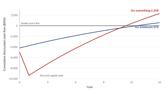
Ridgeline Water's finance department has told the project to use a real discount rate of 5 % for its base case and to test 7 %. The code below computes NPV, a benefit–cost ratio and payback for both options.
def npv(rate, flows):
    return sum(cf / (1 + rate) ** t for t, cf in enumerate(flows))

def payback(flows):
    cum = 0.0
    for t, cf in enumerate(flows):
        prev = cum
        cum += cf
        if cum >= 0 and t > 0:
            return t - 1 + (-prev / cf)
    return None

years = 15
# incremental cash flows against do nothing, $000
dmin = [-4200] + [520 - 60] * years
dsom = [-5000, -4600] + [1420 - 180] * (years - 1)
for name, f in [("do minimum", dmin), ("do something", dsom)]:
    pv_costs = -sum(cf / 1.05 ** t for t, cf in enumerate(f) if cf < 0)
    pv_ben = sum(cf / 1.05 ** t for t, cf in enumerate(f) if cf > 0)
    print(f"{name:13} NPV@5% {npv(0.05, f):6.0f}  NPV@7% {npv(0.07, f):6.0f}  "
f"BCR {pv_ben / pv_costs:4.2f} payback {payback(f):4.1f} yr")do minimum NPV@5% 575 NPV@7% -10 BCR 1.14 payback 9.1 yr do something NPV@5% 2309 NPV@7% 836 BCR 1.25 payback 8.7 yr
At 5 %, the smart-meter option has an NPV of about 2.3 million, four times that of the drive-by option, and a benefit–cost ratio of 1.25 against 1.14. At 7 %, the drive-by option's NPV falls to roughly zero while the smart-meter option still shows about 0.8 million. On these figures, do something is preferred at both rates. The payback periods are similar, about 8.7 and 9.1 years, which shows why payback alone would not distinguish the options well.
Internal rate of return
The internal rate of return (IRR) is the discount rate at which an option's NPV is exactly zero. It is often quoted because it is a single percentage that can be compared with the organization's required rate. For the smart-meter option the IRR is about 8.4 %; for the drive-by option it is about 7.0 %. Both exceed the 5 % base rate, so both have positive NPVs at that rate. IRR has known pitfalls: options with unusual cash flow patterns can have several IRRs, and IRR does not show the scale of value created. When options are mutually exclusive, NPV at the organization's rate is the safer basis for choice.
| Measure | Do minimum | Do something | What it tells the board |
|---|---|---|---|
| Simple payback | 9.1 years | 8.7 years | How long the money is at risk |
| NPV at 5 % | About 575 | About 2,309 | Value created at the organization's rate |
| NPV at 7 % | About −10 | About 836 | Robustness to a higher rate |
| Benefit–cost ratio at 5 % | 1.14 | 1.25 | Value per dollar of cost |
| IRR | About 7.0 % | About 8.4 % | Rate at which NPV is zero |
Sensitivity analysis
Every figure in an appraisal is a forecast, and some forecasts matter more than others. Sensitivity analysis changes one assumption at a time to see how much the result moves. It identifies which assumptions the decision really rests on, so that the board can focus scrutiny and risk management there. A related idea is the break-even value: how far an assumption can move before the option stops creating value.
def npv(rate, flows):
    return sum(cf / (1 + rate) ** t for t, cf in enumerate(flows))

base = {"reading": 380, "billing": 150, "leaks": 640, "energy": 250}
op_cost, capex = 180, [-5000, -4600]

def flows(ben, capex=capex, delay=0):
    net = sum(ben.values()) - op_cost
    return capex + [0] * delay + [net] * (14 - delay)

print("case                         NPV@5% ($000)")
print(f"{'base':28} {npv(0.05, flows(base)):8.0f}")
low = dict(base, leaks=base["leaks"] * 0.5)
print(f"{'leak benefit halved':28} {npv(0.05, flows(low)):8.0f}")
print(f"{'capital cost +20 %':28} {npv(0.05, flows(base, [c * 1.2 for c in capex])):8.0f}")
print(f"{'benefits start 1 yr late':28} {npv(0.05, flows(base, delay=1)):8.0f}")
print(f"{'all benefits -20 %':28} {npv(0.05, flows({k: v * 0.8 for k, v in base.items()})):8.0f}")
lo, hi = 0.0, 1.0
for _ in range(50):
    mid = (lo + hi) / 2
    if npv(0.05, flows({k: v * mid for k, v in base.items()})) < 0:
        lo = mid
    else:
        hi = mid
print(f"break-even benefit level: {hi:.0%} of forecast")case NPV@5% ($000) base 2309 leak benefit halved -708 capital cost +20 % 433 benefits start 1 yr late 1184 all benefits -20 % -368 break-even benefit level: 83% of forecast
The results are sobering. The option survives a 20 % capital cost overrun and a one-year delay in benefits, but it turns negative if the leak saving is only half what is forecast, or if all benefits come in 20 % low. The break-even point is about 83 % of forecast benefits, which leaves little margin. The leak saving is the largest single benefit and the one most dependent on customers acting on alerts, so it is where the board should focus. Possible responses include a pilot in one district to measure leak savings before full rollout, or staging the rollout so that later stages can be stopped if the benefit does not appear.
| Assumption | Effect on NPV at 5 % | Implication for the project |
|---|---|---|
| Leak saving halved | Falls from about 2,309 to about −708 | Critical: pilot and measure before committing to full rollout |
| All benefits 20 % lower | Falls to about −368 | Benefits need firm owners and measures |
| Capital cost 20 % higher | Falls to about 433 | Tolerable, but cost tolerance should be tight |
| Benefits start a year late | Falls to about 1,184 | Tolerable; time tolerance can be moderate |
This is where the business case connects to the plans and organizing practices. A pilot stage changes the plan; tight cost tolerance shapes the stage plans; and the benefit owners named by the senior user become accountable for the leak saving. Investment appraisal is not an end in itself; it tells the project where its control effort will matter most.
Risk-adjusted appraisal
Sensitivity analysis changes one thing at a time. A risk-adjusted appraisal weighs scenarios by their likelihood. In the simplest form, the expected NPV is the probability-weighted average of scenario NPVs. Suppose the board judges a 60 % chance that the base case holds and a 40 % chance that the leak saving is only half the forecast. The expected NPV is then 0.6 × 2,309 + 0.4 × (−708) ≈ 1,102 thousand.
An expected NPV of about 1.1 million is still positive, but the 40 % chance of a loss matters to an organization that cannot absorb one easily. Expected value does not capture the organization's appetite for risk, which is why PRINCE2 links the business case to the risk practice and to the risk appetite set by the business layer. PRIN-131 covers risk in detail.
Worked problem
Valuing a pilot stage
A three-month pilot in one district would cost 300 thousand and would reveal whether the leak saving is closer to the base case or to half. If the pilot shows the low case, the board would stop after the pilot and avoid the loss; if it shows the base case, the full project goes ahead. Using the 60/40 probabilities and ignoring the small delay, is the pilot worth doing?
Show solution
- Without the pilot: expected NPV ≈ 1,102.
- With the pilot: 60 % chance of proceeding with NPV 2,309; 40 % chance of stopping with NPV 0; less the pilot cost of 300.
- Expected NPV with pilot ≈ 0.6 × 2,309 + 0.4 × 0 − 300 = 1,385 − 300 = 1,085.
- The expected values are almost equal, but the pilot removes the 40 % chance of a 708 thousand loss.
Answer: On expected value alone the two choices are about the same, but the pilot sharply reduces downside risk. A cautious board would likely choose it, and it would become the first management stage after initiation.
Non-financial benefits and qualitative factors
Not everything can sensibly be converted into money. Ridgeline Water's smart meters may improve customer trust, support water conservation targets and give planners better data. These benefits should still appear in the business case with measures, even if they are not in the NPV. Equally, some dis-benefits, such as privacy concerns about detailed consumption data, are qualitative. The board must weigh them alongside the numbers. A business case that presents only an NPV hides judgments that the board should make openly.
| Benefit or dis-benefit | Monetized? | Possible measure |
|---|---|---|
| Reduced reading cost | Yes | Reading cost per connection per year |
| Fewer billing disputes | Partly | Disputes per 1,000 bills; handling cost |
| Customer trust | No | Annual survey score on billing accuracy |
| Water conservation | Partly | Litres per connection per day |
| Privacy concerns | No | Complaints received; opt-out requests |
Common mistakes
MistakeRelying on payback alone.
InsteadUse payback alongside NPV, which counts all benefits and the time value of money.
MistakeChoosing a discount rate inside the project to make the case look good.
InsteadUse the rate set by the organization and test sensitivity to other rates.
MistakeChoosing between exclusive options by IRR alone.
InsteadCompare NPVs at the organization's rate; IRR ignores scale and can mislead.
MistakePresenting one NPV without sensitivity analysis.
InsteadShow which assumptions the decision rests on and their break-even values.
MistakeLeaving out benefits that cannot be monetized.
InsteadRecord them with measures and let the board weigh them explicitly.
Summary and key terms
- Investment appraisal compares options' costs and benefits over time against the do nothing baseline.
- Payback shows how long money is at risk but ignores later benefits and discounting.
- NPV discounts future cash flows at the organization's rate; a higher NPV is preferred.
- IRR is the rate at which NPV is zero; use NPV to choose between exclusive options.
- Sensitivity analysis and break-even values show which assumptions matter most.
- Risk-adjusted appraisal weighs scenarios; a pilot stage can reduce downside risk.
- Non-financial benefits and dis-benefits should be measured and weighed, not ignored.
- Investment appraisal
- A comparison of an option's costs and benefits over time to judge its value.
- Payback period
- The time for cumulative net benefits to recover the initial cost.
- Discount rate
- The rate used to convert future cash flows into present values.
- Net present value
- The sum of an option's discounted cash flows.
- Benefit–cost ratio
- The present value of benefits divided by the present value of costs.
- Internal rate of return
- The discount rate at which an option's net present value is zero.
- Sensitivity analysis
- Changing one assumption at a time to see how much the result moves.
- Break-even value
- The value of an assumption at which an option's net present value becomes zero.
- Expected value
- The probability-weighted average of possible outcomes.
- Appraisal period
- The number of years over which costs and benefits are compared.
Practice problems
Work each problem on paper first, then reveal the answer to check.
An option costs 600 and saves 150 a year. Simple payback?
Show answer
4 years.
What is the present value of 1,000 received in 2 years at 5 %?
Show answer
About 907.
Why might two options with similar payback have very different NPVs?
Show answer
Payback ignores benefits after the payback point and the time value of money.
Who normally sets the discount rate?
Show answer
The organization, not the project.
An option's IRR is 8 % and the organization's rate is 5 %. Is its NPV at 5 % positive?
Show answer
Yes.
What does a break-even benefit level of 83 % tell you?
Show answer
The option stops creating value if benefits fall below 83 % of forecast.
Scenarios: 70 % chance NPV 1,000; 30 % chance NPV −500. Expected NPV?
Show answer
550.
Why might a board choose a pilot with a slightly lower expected NPV?
Show answer
It reduces the chance of a large loss.
Give one non-monetized benefit of smart meters.
Show answer
Improved customer trust or better planning data.
Which practice addresses the organization's appetite for risk in more depth?
Show answer
The risk practice.
Lesson quiz · 5 questions
Score 60% or more to complete this lesson.
Create a free account to save your progress, take quizzes and earn a certificate.