
PET-460 · Lesson 5 of 12 · 20 min
CO2 pipelines and transport
Sofia Reyes had built gas gathering systems and a sales line for Prairie Crest, and her first sketch of the hub's transport system looked familiar: lateral lines from each capture plant to a compressor station, and a trunk line 110 km (70 miles) to the storage site. The differences emerged as soon as she started the calculations. “Natural gas lines are sized for velocity and compression cost,” she told Ethan. “A CO₂ line also has to stay in one phase from end to end, survive a rupture without the crack running for kilometres, and protect people from a heavy, invisible gas that collects in low ground. Each of those sets a number in the design.”
Conditioning and compression
CO₂ leaves an amine stripper at about 150 to 200 kPa, saturated with water and at about 40 °C. Raising it to pipeline pressure, 15 MPa (2,175 psia) for the hub, is done in two parts. A multistage compressor, often an integrally geared machine with four to eight stages and intercoolers, raises it to just above the critical pressure; each intercooler condenses water, and a dehydration unit, usually triethylene glycol (TEG) contact or molecular sieves, between the middle stages brings water down to the specification of Lesson 4. Once the CO₂ is dense, a pump completes the pressure rise at much lower energy, because pumping a liquid-like fluid needs far less work than compressing a gas. Compression and pumping together take about 90 to 110 kWh per tonne for a low-pressure source, and less for sources that deliver CO₂ at higher pressure, such as the flash stages of a pre-combustion plant.
For the hub, Sofia proposed a compressor at each large source and a central pump station at the head of the trunk line. Smaller sources would send compressed CO₂ through short laterals. Electrical power for compression became one of the hub's largest operating costs: about 30 MW for 3 million tonnes a year. Its emissions, from the Alberta grid, are part of the avoided-CO₂ calculation of Lesson 1.
# CO2 trunk line: compression power, line size, pressure profile and booster spacing (dense phase).
import math
SI = True      # True: Canadian hub trunk line, metric; False: US hub trunk line, US units

rate = 3.0e9 / (8760 * 3600)            # kg/s for 3.0 Mt/yr at steady flow
rho, mu, eps = 860.0, 7.5e-5, 4.5e-5    # kg/m3, Pa s, m (dense CO2 at ~10 C and 10-15 MPa; illustrative)
L_km = 110.0 if SI else 113.0           # trunk length
dz = 60.0 if SI else -15.0              # net elevation gain along the line, m
p_in, p_min = 15.0e6, 10.0e6            # Pa: discharge, and the minimum kept to stay well above the critical pressure

def friction(Re, d):                    # Swamee-Jain explicit form of Colebrook
    return 0.25 / math.log10(eps / (3.7 * d) + 5.74 / Re ** 0.9) ** 2

def dp_per_m(d):
    v = rate / rho / (math.pi * d * d / 4); Re = rho * v * d / mu
    return friction(Re, d) * rho * v * v / (2 * d), v, Re

# compression: 5 intercooled stages from 0.15 MPa to 7.5 MPa (ideal gas, k = 1.29), then a dense-phase pump to 15 MPa
k, eta, T1 = 1.29, 0.80, 313.15
ratio = (7.5 / 0.15) ** (1 / 5)
w_stage = k / (k - 1) * 8.314 / 0.04401 * T1 * (ratio ** ((k - 1) / k) - 1) / eta     # J/kg per stage
w_comp = 5 * w_stage / 3.6e6 * 1000                     # kWh/t
w_pump = (15.0e6 - 7.5e6) / (rho * 0.75) / 3.6e6 * 1000
print(f"Compression {w_comp:.0f} kWh/t + pumping {w_pump:.0f} kWh/t = {w_comp + w_pump:.0f} kWh/t; "
      f"{(w_comp + w_pump) * rate * 3.6 / 1000:.1f} MW for {rate:.1f} kg/s")

sizes = [("NPS 12", 0.3048, 0.0103), ("NPS 16", 0.4064, 0.0127), ("NPS 20", 0.5080, 0.0143)]
print(f"\nTrunk line {L_km:.0f} km ({L_km / 1.609:.0f} mi), net rise {dz:.0f} m")
for name, od, wt in sizes:
    d = od - 2 * wt; g, v, Re = dp_per_m(d)
    loss = g * L_km * 1000 + rho * 9.81 * dz
    reach = (p_in - p_min - rho * 9.81 * dz) / g / 1000 if g > 0 else float('inf')
    if SI: print(f"{name}: v {v:.2f} m/s, Re {Re:,.0f}, drop {g:.1f} kPa/km, outlet {(p_in - loss) / 1000:,.0f} kPa, reach to 10 MPa {reach:,.0f} km")
    else:  print(f"{name}: v {v * 3.281:.1f} ft/s, drop {g * 1609 / 6894.8:.1f} psi/mi, outlet {(p_in - loss) / 6894.8:,.0f} psia, reach to 1,450 psia {reach / 1.609:,.0f} mi")
# booster spacing for a hypothetical extension of the same NPS 12 line to 400 km (250 mi)
d = sizes[0][1] - 2 * sizes[0][2]; g = dp_per_m(d)[0]
spacing = (p_in - p_min) / g / 1000
n_pumps = math.ceil(400 / spacing) - 1
if SI: print(f"\nNPS 12 extended to 400 km: a booster every {spacing:.0f} km, so {n_pumps} intermediate pump stations")
else:  print(f"\nNPS 12 extended to 250 mi: a booster every {spacing / 1.609:.0f} mi, so {n_pumps} intermediate pump stations")
g16 = dp_per_m(0.4064 - 0.0254)[0]
pts = [(x, p_in - g16 * x * 1000 - rho * 9.81 * dz * x / L_km) for x in [L_km * i / 5 for i in range(6)]]
if SI: print("Pressure profile, NPS 16:", ", ".join(f"{x:.0f} km {p / 1e6:.2f} MPa" for x, p in pts))
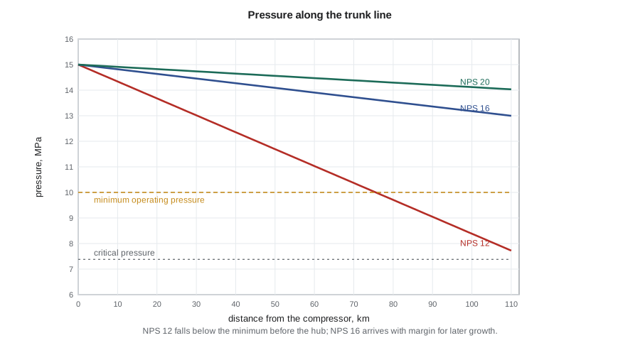
else: print("Pressure profile, NPS 16:", ", ".join(f"{x / 1.609:.0f} mi {p / 6894.8:,.0f} psia" for x, p in pts))Compression 88 kWh/t + pumping 3 kWh/t = 91 kWh/t; 31.2 MW for 95.1 kg/s Trunk line 110 km (68 mi), net rise 60 m NPS 12: v 1.74 m/s, Re 5,682,500, drop 61.6 kPa/km, outlet 7,723 kPa, reach to 10 MPa 73 km NPS 16: v 0.97 m/s, Re 4,238,757, drop 13.6 kPa/km, outlet 12,997 kPa, reach to 10 MPa 330 km NPS 20: v 0.61 m/s, Re 3,368,724, drop 4.2 kPa/km, outlet 14,032 kPa, reach to 10 MPa 1,072 km NPS 12 extended to 400 km: a booster every 81 km, so 4 intermediate pump stations Pressure profile, NPS 16: 0 km 15.00 MPa, 22 km 14.60 MPa, 44 km 14.20 MPa, 66 km 13.80 MPa, 88 km 13.40 MPa, 110 km 13.00 MPa
Hydraulics of dense-phase lines
In the dense phase, CO₂ flows like a liquid and the line is sized with the Darcy-Weisbach equation:
The Colebrook equation (or its explicit Swamee-Jain approximation, used in the code) gives the friction factor from the Reynolds number and relative roughness. Dense CO₂ has a high density and a low viscosity, so Reynolds numbers are in the millions and flow is fully turbulent. Unlike a gas line, the density hardly changes along the line, so velocity is nearly constant, and elevation matters: a 60 m (200 ft) rise costs about 0.5 MPa (75 psi) of head, as it would for water.
Two pressure limits frame the design. The maximum is the line's maximum operating pressure, set by pipe grade, wall thickness and the design code, and limited in practice by the compressor discharge. The minimum is the pressure needed to stay safely in the dense phase all the way to the delivery point, including the bubble point of the impure stream and a margin; for the hub, 10 MPa (1,450 psia). The allowed pressure drop, 5 MPa (725 psi), divided by the friction gradient gives the maximum distance between pump stations. For the 110 km trunk line, an NPS 12 pipe would drop below the minimum before reaching the hub. An NPS 16 line arrives at about 13 MPa, with enough margin to carry about 5 million tonnes a year later. Larger diameters cost more steel but save pump stations and leave room for growth; for a hub that hopes to attract more sources, Sofia recommended the NPS 16 line.
Worked problem
Pressure drop in a CO₂ lateral
A lateral line 8.0 km (5.0 miles) long carries 0.8 million tonnes a year of CO₂ (25.4 kg/s) at a density of 860 kg/m³ and viscosity 0.075 mPa·s. The pipe is NPS 8 with an inside diameter of 0.203 m and roughness 0.045 mm. Estimate the friction pressure drop.
Show solution
- Velocity: area = π × 0.203² / 4 = 0.0324 m²; volumetric rate = 25.4 / 860 = 0.0295 m³/s; v = 0.91 m/s.
- Reynolds number = 860 × 0.91 × 0.203 / 7.5 × 10⁻⁵ = 2.1 × 10⁶.
- Relative roughness = 0.045 / 203 = 2.2 × 10⁻⁴; Swamee-Jain gives f ≈ 0.0145.
- Δp/L = 0.0145 × 860 × 0.91² / (2 × 0.203) = 25.5 Pa/m = 25.5 kPa/km.
- Over 8.0 km: Δp ≈ 204 kPa.
Answer: The lateral loses about 0.2 MPa (30 psi), a small part of the pressure budget; laterals are sized mainly for future flow and for mechanical strength.
Running fractures and pipe toughness
A rupture in a dense-phase CO₂ line behaves differently from one in a gas line. When the pipe opens, a decompression wave runs along the line at the speed of sound in the fluid. As the pressure falls to the vapour pressure, the CO₂ starts to boil, and the pressure stops falling for a while: the decompression curve has a long plateau near the saturation pressure, higher than for natural gas at the same initial pressure. A crack in the pipe wall travels at a speed set by the steel's toughness and the pressure at the crack tip. If the crack is faster than the pressure falls, it keeps running, potentially for long distances. Preventing that requires steel with high fracture toughness, measured by Charpy impact energy, a lower operating stress (thicker wall), or mechanical crack arrestors, sleeves fitted at intervals that stop a running crack. Impurities make it worse, because they raise the saturation plateau. The Battelle two-curve method, developed for gas lines and adapted for CO₂ with full-scale burst tests, is the standard way to check the design.
Codes and regulation
In Canada, CO₂ pipelines are designed to CSA Z662, Oil and gas pipeline systems, which has a clause for CO₂, and in Alberta the AER licenses and inspects them under the Pipeline Act. Lines that cross provincial or international borders fall under the Canada Energy Regulator. The Alberta Carbon Trunk Line, about 240 km of 16-inch pipe built for up to 14.6 million tonnes a year, is the country's largest example. Codes set design factors, material requirements, valve spacing, leak detection, integrity management and emergency planning.
The 2020 rupture of a CO₂ pipeline near Satartia, Mississippi, changed the debate. Heavy rain caused a landslide that broke a line operated by Denbury. The plume of cold CO₂ flowed into the village, about 200 people were evacuated and at least 45 were treated in hospital; vehicle engines stalled for lack of oxygen, slowing the response. Emergency responders had not been told what the pipeline carried or how to respond. PHMSA's investigation led to a notice to operators about geohazards and, in January 2025, a proposed rule covering CO₂ in all phases, dispersion modelling, emergency planning and notification of local responders. The proposal was withdrawn under the new administration's regulatory freeze shortly afterward, so US federal rules remain as before, though several states have added their own requirements and the lessons inform design everywhere. Alberta's requirements and CSA Z662 already require emergency response planning for CO₂ lines; the hub adopted the Satartia lessons in its own plan.
Dispersion and routing
CO₂ is not flammable, but it is an asphyxiant and, at high concentration, toxic: above about 5 percent in air it causes headaches and breathing difficulty, and above about 10 percent loss of consciousness within minutes. Because it is heavier than air, a large release flows along the ground and collects in valleys, ditches and basements, especially in calm weather. Dispersion modelling for a pipeline route therefore considers terrain, not just distance, and identifies low areas where a plume could pool. Routing avoids running a line uphill of communities where possible, places block valves to limit the inventory that can escape from any section, and adds detection and notification. CO₂ contains no odorant; adding one has been studied but is not standard. The hub's route along existing pipeline corridors in Alberta's Industrial Heartland crossed mostly flat farmland, with one river valley that Sofia flagged for detailed modelling.
| Concentration of CO₂ in air | Effect (approximate) |
|---|---|
| 0.04% (400 ppm) | normal outdoor air |
| 0.5% (5,000 ppm) | typical occupational exposure limit over a work shift |
| 3–5% | faster breathing, headache, impaired judgement with exposure |
| 7–10% | dizziness, loss of consciousness within minutes to an hour |
| above 10–15% | rapid loss of consciousness; potentially fatal |
Ships, trucks and rail
Not every source is near a pipeline. Ships carry CO₂ as a cold liquid, at about −50 °C and 0.7 MPa (100 psia) in low-pressure designs or −30 °C and 1.5 to 2 MPa (220 to 290 psia) in medium-pressure ones, and have long served the food and beverage industry on a small scale. The Northern Lights project in Norway, which began injecting in 2025, receives CO₂ by ship at a coastal terminal and pipes it offshore to a saline formation, and several European hubs plan to collect CO₂ from many coastal emitters the same way. Ship transport has lower capital cost and more flexibility than a pipeline but higher operating cost per tonne, and it requires liquefaction, buffer storage and terminals. Trucks and rail suit small volumes, such as an ethanol plant's fermentation CO₂ before a pipeline is available. For the hub, all four sources were within pipeline distance, but Lena wanted the storage site to keep land for a future truck or rail unloading facility.
Common mistakes
MistakeSizing a CO₂ line as if it were a natural gas line.
InsteadDense CO₂ behaves like a liquid: elevation and friction dominate, density is nearly constant, and the minimum pressure is set by phase behaviour.
MistakeUsing natural gas toughness requirements for CO₂ pipe.
InsteadCheck running fracture with the CO₂ decompression curve for the actual impurities; specify toughness, wall thickness or crack arrestors.
MistakeModelling a release with distance-only setbacks.
InsteadModel dispersion with terrain; CO₂ flows downhill and pools in low ground.
MistakeLeaving local responders uninformed about what the line carries.
InsteadShare the hazard, the dispersion zones and the response plan with communities and emergency services.
Summary and key terms
- CO₂ is compressed in stages with intercooling and dehydration, then pumped once dense; about 90 to 110 kWh per tonne in total.
- Dense-phase lines are sized with Darcy-Weisbach friction and elevation; the pressure must stay above the impure stream's bubble point plus a margin.
- Pump station spacing equals the allowed pressure drop divided by the friction gradient.
- CO₂ decompression has a high plateau, so pipe toughness or crack arrestors must stop running fractures.
- Released CO₂ is heavy and odourless and pools in low ground; dispersion modelling, routing and responder notification are essential.
- Ships and trucks carry cold liquid CO₂ for sources without pipeline access.
- Dense-phase pipeline
- A pipeline operating with CO₂ in liquid or supercritical form.
- Minimum operating pressure
- The lowest pressure allowed in the line to keep the stream single-phase with margin.
- Running fracture
- A crack that propagates along a pipeline after rupture because the fluid pressure at the crack tip stays high.
- Crack arrestor
- A sleeve or ring fitted to a pipeline to stop a running fracture.
- Decompression wave
- The pressure disturbance that travels along a ruptured pipeline at the speed of sound in the fluid.
- Dispersion modelling
- Prediction of where and at what concentration a released gas travels.
Practice problems
Work each problem on paper first, then reveal the answer to check.
A trunk line loses 14 kPa/km (3.2 psi/mi). The allowed drop between stations is 5 MPa (725 psi). What is the maximum spacing between pump stations?
Show answer
5,000 / 14 ≈ 360 km.
Why is elevation more important for a CO₂ line than a gas line?
Show answer
Dense CO₂ has a liquid-like density, so the hydrostatic head of a rise is large.
What feature of CO₂ decompression makes running fractures a concern?
Show answer
The pressure plateau at the saturation pressure during boiling keeps the crack-tip pressure high.
Give two measures that reduce the hazard of a CO₂ pipeline release.
Show answer
Block valves to limit inventory; routing away from low ground near communities; dispersion modelling; responder notification and detection.
Lesson quiz · 5 questions
Score 60% or more to complete this lesson.
Create a free account to save your progress, take quizzes and earn a certificate.