Steamflooding

Prairie Crest's board has asked the thermal group to look at a second kind of asset: a heavy oil lease in western Saskatchewan near Lloydminster, where the oil is far less viscous than Wapiti Lake bitumen and a continuous steamflood between vertical or deviated wells could work. Mei Lin, the company's planning manager, wants a first estimate within a month. 'The geologists say the sand is about 18 m thick,' she tells Ethan. 'Our partners in California have run steamfloods for decades. Find out how they think about it.'

This lesson explains continuous steamflooding: how steam drives oil from injectors to producers, the well patterns used, how the heated zone grows and how much heat is lost to the surrounding rock, using the classic Marx-Langenheim model. It ends with the stages of a mature flood and the giant California fields where the process was developed.

How a steamflood works

In a steamflood, steam is injected continuously into some wells and oil is produced from others nearby. Around each injector, a steam zone forms in which the temperature is close to the steam temperature and the oil saturation falls to a low residual value, often 10 to 15 percent, because hot oil is very mobile and part of it is distilled by the steam. Ahead of the steam zone is a hot water zone, where condensed steam pushes heated oil toward the producers, and beyond that a cold zone with an oil bank. Oil is displaced by the advancing steam and hot water, by viscosity reduction, by steam distillation of the lighter components and, in thick sands, by gravity drainage from the top of the oil column.

Because steam is much less dense than oil and water, it tends to rise to the top of the sand and flow along it, a behaviour called steam override or gravity override. Override reduces the vertical sweep but also brings heat into contact with oil in the upper part of the sand, which then drains downward. In thick, high-permeability sands, the process becomes partly a gravity drainage process, and operators often complete injectors only in the lower part of the sand to make the best use of override.

Patterns

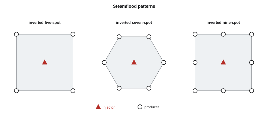
Steamfloods are usually arranged in repeated patterns. The inverted five-spot has an injector at the centre of a square with four producers at the corners; the inverted seven-spot and nine-spot use six or eight producers around each injector. Pattern sizes are small compared with waterfloods, because the heat must travel between wells before too much of it is lost: about 1 to 2 ha (2.5 to 5 acres) per pattern is typical in California, and some floods use smaller patterns still. Many floods start as cyclic steam projects in which every well is steamed, and are then converted to a continuous flood by turning some wells into injectors.

The Marx-Langenheim model

In 1959 J. W. Marx and R. H. Langenheim published a simple model of a heated zone growing in a reservoir layer while losing heat by conduction to the cap and base rock. They assumed that the heated zone is at the steam temperature throughout, that heat is injected at a constant rate and that the heat conducts vertically into the overburden and underburden. The heated area after time t is

Here Q is the rate of heat injected into the sand, M_R and M_ob are the volumetric heat capacities of the reservoir and of the surrounding rock, k_ob is the thermal conductivity of the surrounding rock, h the heated thickness and ΔT the temperature rise. The thermal efficiency, the fraction of the injected heat that is still in the reservoir, is G(t_D)/t_D. It starts near 100 percent and falls with time, faster in thin sands, because the area of hot rock in contact with the cap and base rock grows while the volume of sand per unit area is fixed.

# Marx-Langenheim heated area for a steamflood pattern
import math
SI = True   
def erfc(x): return math.erfc(x)
def F(tD):
    # G(tD) = exp(tD) erfc(sqrt tD) + 2 sqrt(tD/pi) - 1 ; area A = Q M h G / (4 kh_ob M_ob dT) (consistent units)
    return math.exp(tD) * erfc(math.sqrt(tD)) + 2 * math.sqrt(tD / math.pi) - 1
# SI inputs
h = 18.0                    # m net heated thickness
Mr = 2.6e6                  # J/(m3 K) reservoir heat capacity
Mob = 2.4e6                 # J/(m3 K) cap and base rock
k_ob = 1.7                  # W/(m K) cap and base rock conductivity
a_ob = k_ob / Mob           # m2/s
dT = 260.0 - 30.0           # K
Q = 5.0e6                   # W of heat into the sand (about 160 t/d of 70 % steam after wellbore losses)
for years in (0.5, 1, 2, 4, 8):
    t = years * 365.25 * 86400
    tD = 4 * k_ob * Mob * t / (Mr ** 2 * h ** 2)
    A = Q * Mr * h * F(tD) / (4 * k_ob * Mob * dT)
    eff = F(tD) / tD          # thermal efficiency: fraction of injected heat still in the sand
    if SI: print(f"{years:4.1f} years: heated area {A / 1e4:5.2f} ha, heat still in the sand {eff:.0%}")
    else:  print(f"{years:4.1f} years: heated area {A / 4046.9:5.2f} acres, heat still in the sand {eff:.0%}")

 0.5 years: heated area  0.58 ha, heat still in the sand 79%
 1.0 years: heated area  1.06 ha, heat still in the sand 73%
 2.0 years: heated area  1.90 ha, heat still in the sand 65%
 4.0 years: heated area  3.31 ha, heat still in the sand 56%
 8.0 years: heated area  5.56 ha, heat still in the sand 47%

With 5 MW of heat entering an 18 m (59 ft) sand, the model gives a heated area of about 1.1 ha (2.6 acres) after one year and 5.6 ha (13.7 acres) after eight. Over the same time the share of the heat still in the sand falls from 73 to 47 percent. Ethan notices the second result first. 'Half the heat ends up in the cap and base rock?' he asks. 'In a thin sand, yes, eventually,' Lena replies. 'That is why thickness matters so much in thermal recovery, and why we cut steam back as a flood matures.'

The model is approximate. It ignores the hot water zone ahead of the steam, steam override and the distribution of heat across a real pattern, and it assumes a constant injection rate. More detailed models, such as those of Mandl and Volek, which allow for the hot water zone after a critical time, and full thermal simulation are used for design. But Marx-Langenheim remains a quick way to estimate how fast the heated zone will grow and how efficient the process will be.

Oil recovery and steam-oil ratio

If the heated zone sweeps a known area, the oil displaced is roughly that area times the thickness, porosity and the change in oil saturation from initial to residual in the steam zone, adjusted for a capture efficiency at the producers. Dividing the steam injected by that oil gives an estimate of the SOR. In practice the SOR of a California steamflood is typically about 3 to 5 in the main phase, rising as the flood matures. Ultimate recoveries of 50 to 70 percent of the original oil in place are achieved in the best floods, far higher than the 5 to 10 percent typical of primary production in the same reservoirs.

A flood's life cycle

A steamflood moves through recognisable stages. In the early stage, steam injection rates are high, the steam zone grows rapidly and oil rates rise as the oil bank reaches the producers. In the main stage, the oil rate is near its peak and the SOR is relatively low. Once steam breaks through to the producers, further heat injection mostly heats rock and water already swept; operators then reduce steam rates, switch to injecting hot water or unheated water, or stop injection and let the heat already in the reservoir continue to drain oil. This heat management, often called steam-cut or wind-down, can greatly reduce the SOR in the late life of a flood.

Infill drilling is also common. Adding wells between existing ones shortens the distance heat must travel, reaches oil that the original pattern left behind and is often the cheapest way to add production to a mature flood. Horizontal wells drilled near the base of the sand in old floods can collect oil that drains down from the heated upper part.

The California steamfloods

Steamflooding was developed largely in California. The first significant steam drive tests were run in the 1960s in fields such as Kern River and Midway-Sunset in Kern County, and by the 1980s steam-based production made up a large share of the state's oil. The Kern River field, discovered in 1899 near Bakersfield, has produced more than two billion barrels, most of it with steam, and Midway-Sunset has produced even more. In Canada, steamflooding has been used in Saskatchewan's heavy oil, for example at the Pikes Peak project near Lloydminster from the early 1980s, and as a follow-up to cyclic steam at Cold Lake.

Monitoring a steamflood

A steamflood is monitored with observation wells, temperature surveys and production tests. Observation wells, often cased with fibreglass or steel and fitted with thermocouples, show the temperature profile through the sand and how it changes as the steam zone grows. Saturation logs run through casing, such as pulsed neutron or carbon-oxygen logs, show where oil has been swept and where it remains. Producers are tested regularly to measure oil, water and gas rates, and their temperatures show which ones are close to the steam front. Combined with the injection rates, these data let engineers estimate how much of each pattern has been heated and how efficiently heat is being used.

Engineers also carry out heat balances: comparing the heat injected with the heat produced in hot fluids and the heat estimated to remain in the reservoir and in the cap and base rock. A pattern in which much more heat is going in than the steam zone growth can account for may be losing steam to a thief zone or to a neighbouring pattern, and its injection is reduced or redirected.

Steam distribution between injectors

A steamflood field may have hundreds of injectors fed from a few steam generators through a network of pipelines. Delivering the right amount of steam of the right quality to each injector is difficult, because steam and water tend to split unequally at pipe junctions, so some injectors receive wetter steam than others. Operators use flow control devices, chokes sized for critical flow and steam separators at key points, and measure the steam quality at major branches. Steam distribution is a frequent target for improvement, because steam that arrives at the wrong place or in the wrong form represents fuel spent with no oil to show for it.

Late-life recovery

Even mature floods hold large volumes of oil. Residual oil saturation in the steam zone is low, but the unswept parts of patterns, the lower part of the sand under the steam zone and areas between patterns may still contain much of their original oil. Late-life strategies include drilling horizontal wells near the base of the sand to collect oil draining from above, redistributing steam to less-swept areas, injecting hot water to scavenge heat and oil, and testing solvents or other additives. Each is evaluated on its incremental oil per unit of cost and emissions, because in the late life of a flood the margin between a profitable and an unprofitable barrel is narrow.