
PET-350 · Lesson 12 of 12 · 18 min
Integrated petrophysical evaluation: capstone
Ten weeks after the 100/08-27 delineation well reached total depth, the asset team meets to decide whether to drill more horizontal wells in its part of the Tamarack Lake field. Imogen asks Ethan to present the petrophysical evaluation. 'Put everything together,' she says. 'Shale volume, porosity, saturation, permeability, contacts and net pay, with the uncertainties. Lena needs inputs for her volumetrics, Tom needs rock properties for the completion design, and the managers need to know how confident we are.'
This capstone lesson walks through an integrated petrophysical evaluation of the 100/08-27 delineation well: quality control and depth matching, the interpretation workflow, choosing and testing cutoffs, computing net pay and average properties, the movable hydrocarbon check, uncertainty analysis, and how the results feed the volumetric estimate and the development decision. It draws on every earlier lesson.
Step 1: quality control
Ethan begins by assembling all the data in one project: the wireline logs from both runs, the LWD logs from the pilot hole section, the core data, the formation test pressures and samples, and the mud log. He checks each log against its header for units, mud properties and remarks; depth-matches the second run and the LWD data to the main-run gamma ray, as in lesson 1; shifts the core to the logs using the core gamma scan, as in lesson 11; and flags intervals where the caliper or density correction shows poor hole. A short repeat section confirms that the tools read consistently. Any curve that fails these checks is either corrected or excluded before interpretation begins.
Step 2: the interpretation workflow
Ethan then works through the interpretation in a standard order, using parameters calibrated to core wherever possible.
| Step | Method | Parameters and calibration |
|---|---|---|
| Formation temperature | Geothermal gradient (lesson 2) | Recorded bottomhole temperature |
| Rw | SP and Pickett plot, checked against water analyses (lessons 3 and 7) | Rw = 0.045 ohm·m |
| Shale volume | Gamma ray, Larionov older rocks (lesson 3) | Checked against core X-ray diffraction |
| Porosity | Density with core grain density; neutron-density in gas (lessons 5 and 6) | Core porosity regression |
| Rt | Array induction inversion (lesson 4) | Step-profile model |
| Water saturation | Indonesian, compared with Archie and Simandoux (lessons 7 and 8) | Core m and n; Qv for Waxman-Smits check |
| Permeability | NMR Timur-Coates calibrated to core (lessons 10 and 11) | Core Klinkenberg permeability |
| Contacts | Formation tester gradients (lesson 10) | Free water level; capillary transition from core |
The workflow is iterative. When Ethan compares his log saturations with the saturation-height curves from capillary pressure, they agree within a few saturation units in the upper part of the reservoir but the logs read wetter near the base. He traces the difference to the shale volume method, which overestimates clay in a thin interval with feldspar-rich sand, and corrects it with the spectral gamma ray. Each such check makes the final interpretation more defensible.
Step 3: cutoffs
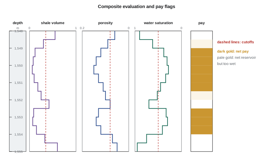
Cutoffs are limits on shale volume, porosity and water saturation that separate rock expected to contribute to production from rock that will not. They are applied in sequence: the shale volume and porosity cutoffs define net reservoir, rock that can store and transmit fluids; the saturation cutoff then defines net pay, net reservoir that holds enough hydrocarbon to produce it economically. A permeability cutoff is sometimes used instead of, or as well as, porosity.
Cutoffs should not be chosen by habit. The porosity cutoff is often tied to a permeability limit through the core porosity-permeability relation: for example, the porosity below which permeability is too low for the planned completion to deliver economic rates. The saturation cutoff can be tied to relative permeability, where water becomes mobile, or to the bulk volume water seen in producing zones. Shale cutoffs relate to the point where shale destroys permeability. For the Cardium, Imogen's team uses shale volume of at most 35 percent, porosity of at least 8 percent and water saturation of at most 50 percent, based on core data and on the performance of the existing horizontal wells.
# Net pay from cutoffs, averaged properties, and hydrocarbon pore thickness for the volumetric estimate
SI = True
step = 0.5 if SI else 1.5           # sample thickness: 0.5 m or 1.5 ft
du = "m" if SI else "ft"
# each sample: (Vsh, porosity, Sw)
samples = [(0.55, 0.06, 0.90), (0.30, 0.09, 0.62), (0.12, 0.12, 0.38), (0.08, 0.14, 0.31), (0.06, 0.15, 0.28),
           (0.10, 0.13, 0.34), (0.18, 0.11, 0.45), (0.25, 0.10, 0.52), (0.42, 0.08, 0.70), (0.09, 0.13, 0.33),
           (0.07, 0.14, 0.30), (0.15, 0.12, 0.41), (0.33, 0.07, 0.75), (0.60, 0.05, 0.95)]
cut = {"Vsh": 0.35, "phi": 0.08, "Sw": 0.50}
gross = len(samples) * step
res = [s for s in samples if s[0] <= cut["Vsh"] and s[1] >= cut["phi"]]
pay = [s for s in res if s[2] <= cut["Sw"]]
h = len(pay) * step
phi_av = sum(s[1] for s in pay) / len(pay)
sw_av = sum(s[1] * s[2] for s in pay) / sum(s[1] for s in pay)    # pore-volume weighted
hpt = sum(s[1] * (1 - s[2]) for s in pay) * step
print(f"gross {gross:.1f} {du}, net reservoir {len(res) * step:.1f} {du}, net pay {h:.1f} {du} (net-to-gross {h / gross:.2f})")
print(f"average porosity {phi_av:.3f}, pore-weighted Sw {sw_av:.2f}, hydrocarbon pore thickness {hpt:.3f} {du}")
for name in ("phi", "Sw"):
    alt = dict(cut); alt[name] = cut[name] + (0.02 if name == "phi" else 0.10)
    p2 = [s for s in samples if s[0] <= alt["Vsh"] and s[1] >= alt["phi"] and s[2] <= alt["Sw"]]
print(f" with {name} cutoff {alt[name]:.2f}: net pay {len(p2) * step:.1f} {du}")gross 7.0 m, net reservoir 5.0 m, net pay 4.0 m (net-to-gross 0.57) average porosity 0.130, pore-weighted Sw 0.34, hydrocarbon pore thickness 0.341 m with phi cutoff 0.10: net pay 4.0 m with Sw cutoff 0.60: net pay 4.5 m
The program applies the cutoffs to the samples across the main reservoir interval of the 100/08-27 delineation well. Of 7.0 m gross, 5.0 m is net reservoir and 4.0 m is net pay, a net-to-gross ratio of 0.57. Average porosity over the pay is 13.0 percent and the pore-volume-weighted water saturation is 34 percent. The hydrocarbon pore thickness, the sum of porosity times hydrocarbon saturation times sample thickness, is about 0.34 m, the single number that best summarizes how much oil the column holds per unit area.
The sensitivity test shows that raising the porosity cutoff to 10 percent does not change net pay here, because the pay samples are well above it, while relaxing the saturation cutoff to 60 percent adds 0.5 m. Net pay is therefore more sensitive to the saturation interpretation than to porosity in this well, which tells the team where further work, such as more capillary pressure measurements, would reduce uncertainty most.
Averages over pay must be weighted correctly. Porosity is averaged by thickness, and water saturation by pore volume, porosity times thickness, because a high-porosity sample holds more fluid than a low-porosity one. Permeability is averaged according to how the layers will flow: arithmetic averages for flow along layers, and harmonic averages across them. Reporting the weighting method is part of a good evaluation.
Step 4: movable hydrocarbon and fluid checks
The flushed-zone saturation from the micro-resistivity Rxo, computed with Rmf, is compared with the uninvaded saturation from Rt, as lesson 4 described. Across the pay, Sxo is 70 to 80 percent while Sw is 30 to 40 percent, showing that the filtrate displaced much of the oil and the oil is movable. NMR free fluid exceeds the hydrocarbon volume, so little free water is expected. The formation tester samples confirm a light oil with a gas-oil ratio close to the field's, and no free gas.
The gas crossover flagged in lesson 6 at the top of the reservoir turns out to be gas released in the flushed zone: the formation test pressures lie on the oil gradient right to the top of the sand, with no gas gradient. Lena is relieved; there is no secondary gas cap at this location. But the pressures are lower than the original pool pressure, confirming that the existing horizontals have depleted this area. That affects the forecast more than any saturation number.
Step 5: uncertainty
Every input to the evaluation carries uncertainty, and the team needs to know how much. Ethan runs the interpretation with low, base and high cases for the most influential parameters: Rw, m and n, the shale volume method, the matrix density and the cutoffs. A more rigorous approach samples all the parameters from probability distributions in a Monte Carlo simulation, recomputing net pay and hydrocarbon pore thickness thousands of times to give a distribution. The result is reported as P90, P50 and P10 values, consistent with the probabilistic reserves categories used by the reservoir engineers (PET-320).
The uncertainty analysis shows that hydrocarbon pore thickness ranges by about plus or minus 20 percent around the base case, dominated by the saturation exponent and the shaly-sand model in the lower part of the reservoir. That range is reported together with the base case.
Step 6: inputs to the volumetric estimate
The results feed directly into the volumetric calculation of PET-320. Original oil in place over an area is the area times the net pay times porosity times hydrocarbon saturation, divided by the oil formation volume factor, or equivalently the area times hydrocarbon pore thickness divided by the formation volume factor. The petrophysical evaluation supplies hydrocarbon pore thickness, net pay and average properties at the well; geologists map them between wells using seismic data and the logs of older wells; and reservoir engineers combine the maps with fluid properties to estimate in-place volumes and their range.
Tom Ashworth takes the rock mechanical properties from the dipole sonic and the core triaxial tests, the stress direction from the image log, and the permeability profile from the calibrated NMR, and uses them to design the completion for the next horizontal wells (PET-330). The production engineers use the permeability and pressures in their inflow models (PET-340).
The recommendation
Ethan's presentation concludes that the Cardium at the 100/08-27 delineation well has 4.0 m of net pay with 13 percent porosity and 34 percent water saturation, comparable to the core of the field, but that reservoir pressure is already depleted by about a fifth. The team recommends drilling two more horizontals from the 08-27 pad, spaced further from the existing wells than in the original plan to limit interference, and coring one of them in the lateral to test the saturation interpretation in the shaly lower interval. The managers approve the plan.
After the meeting, Imogen tells Ethan what she tells every new engineer who rotates through petrophysics. 'The numbers you presented will be used for years by people who never look at the logs. Write down every parameter, every assumption and every calibration, so that someone can check them, and so that you can change them when new data arrive. A petrophysical evaluation is never finished; it is just the best answer so far.'
Worked problem
Net pay and hydrocarbon pore thickness
Five samples, each 0.5 m thick, have (Vsh, φ, Sw) of (0.10, 0.14, 0.30), (0.40, 0.09, 0.55), (0.15, 0.12, 0.40), (0.05, 0.15, 0.28) and (0.20, 0.07, 0.60). With cutoffs Vsh ≤ 0.35, φ ≥ 0.08 and Sw ≤ 0.50, find net pay and hydrocarbon pore thickness.
Show solution
- Sample 2 fails shale volume and saturation; sample 5 fails porosity and saturation. Samples 1, 3 and 4 pass.
- Net pay = 3 × 0.5 = 1.5 m.
- Hydrocarbon pore thickness = 0.5 × [0.14 × 0.70 + 0.12 × 0.60 + 0.15 × 0.72] = 0.5 × [0.098 + 0.072 + 0.108] = 0.139 m.
Answer: Net pay is 1.5 m and the hydrocarbon pore thickness is about 0.14 m.
Documenting the evaluation
The final deliverable is a petrophysical report: the data inventory and quality notes, the depth shifts, every parameter with its source, the equations used, the cutoffs and their basis, the results interval by interval, the uncertainty cases and the comparison with core, tests and nearby wells. A digital file of the computed curves accompanies it. In regulated reserves reporting, the qualified evaluator relies on such documentation, and auditors check it. Good documentation also means the next interpreter can start from this work rather than repeat it.
Common mistakes
MistakeStarting interpretation before quality control and depth matching.
InsteadCheck headers, depths and hole conditions first.
MistakeChoosing cutoffs by habit.
InsteadTie cutoffs to core permeability, relative permeability and production performance.
MistakeAveraging water saturation by thickness.
InsteadWeight saturation by pore volume.
MistakeReporting a single net pay without uncertainty.
InsteadReport low, base and high cases or a probability distribution.
MistakeIgnoring pressure data in a saturation evaluation.
InsteadPressures show contacts, depletion and connectivity that logs cannot.
Summary and key terms
- An integrated evaluation starts with quality control and depth matching of all data.
- The workflow calculates temperature, Rw, shale volume, porosity, Rt, saturation, permeability and contacts, calibrated to core.
- Cutoffs on shale volume, porosity and saturation define net reservoir and net pay and should be tied to rock and production data.
- Hydrocarbon pore thickness summarizes the hydrocarbon column and feeds the volumetric estimate.
- Movable hydrocarbon checks and pressures confirm fluid type, contacts and depletion.
- Uncertainty analysis gives ranges of net pay and hydrocarbon volume for reserves estimates and decisions.
- Cutoff
- A limit on a log-derived property used to define net reservoir or net pay.
- Net reservoir
- Rock that passes shale volume and porosity cutoffs.
- Net-to-gross ratio
- The ratio of net pay or net reservoir thickness to gross thickness.
- Hydrocarbon pore thickness
- The sum of porosity times hydrocarbon saturation times thickness.
- Pore-volume weighting
- Averaging a property by porosity times thickness.
- Monte Carlo simulation
- Repeating a calculation many times with sampled inputs to give a distribution of results.
Practice problems
Work each problem on paper first, then reveal the answer to check.
Why is water saturation averaged by pore volume?
Show answer
High-porosity samples hold more fluid and should count more.
What two cutoffs define net reservoir?
Show answer
Shale volume and porosity.
How does hydrocarbon pore thickness relate to oil in place?
Show answer
OOIP is area times hydrocarbon pore thickness divided by Bo.
Which data showed the crossover was not a gas cap?
Show answer
Formation pressures lying on the oil gradient to the top of the sand.
Lesson quiz · 5 questions
Score 60% or more to complete this lesson.
Create a free account to save your progress, take quizzes and earn a certificate.