Volumetric estimates of oil and gas in place

Lena gives Ethan the first task of the study: an independent volumetric estimate of the oil in the Cardium A pool. 'Geology has new maps from the three vertical wells, the 03-22 horizontal and the seismic,' she says. 'Petrophysics has updated porosity and saturation. Before we look at a single production number, I want to know what the static data say. Then, when material balance gives us a different answer, and it will, we'll know which way to look.'

Volumetric estimation is the oldest and most widely used method in reservoir engineering. It needs no production history, so it is the only method available before a pool is developed, and it remains the reference against which performance methods are checked. This lesson covers the volumetric equations for oil and gas, how each input is obtained, and how to express the result as a range rather than a single number.

The volumetric equation for oil

Oil in place is the pore volume of the reservoir rock multiplied by the fraction of that pore volume occupied by oil, converted from reservoir volume to stock-tank volume. The original oil in place, N, is usually written as follows.

Here A is the area of the pool, h the average net pay thickness, φ the average porosity of the net pay, Sw the average water saturation, and Boi the initial oil formation volume factor, which converts reservoir barrels or cubic metres of oil, with its dissolved gas, into stock-tank volume at surface. The product A h is the net rock volume, often called the net pay volume, and A h φ is the pore volume.

In SI units, with A in square metres and h in metres, N comes out in cubic metres of stock-tank oil. Areas are often given in hectares; one hectare is 10,000 m². Oilfield practice in Canada often converts the result to barrels as well, using 1 m³ = 6.29 bbl.

Where the inputs come from

Area and thickness come from maps. Geologists and geophysicists map the top and base of the reservoir from well picks and seismic, and the fluid contacts from pressure data and logs (lesson 1). Net pay is the part of the gross reservoir thickness that is good enough to contribute: it excludes shale beds and rock with too little porosity or permeability, or too much water, using cut-offs agreed between petrophysics and engineering. A net pay isopach map, contoured in thickness, is planimetered or gridded to give the net rock volume.

Porosity comes from logs calibrated to core (PET-250). Each well gives an average over its net pay; a porosity map or a pore-volume map spreads the values across the pool. Water saturation comes from resistivity logs through Archie's equation or from capillary pressure data, and it varies with height above the free water level, so saturation should be averaged with the pore volume as the weight, not the thickness alone.

The formation volume factor comes from the PVT analysis of a reservoir fluid sample (lesson 3). It matters more than it looks: a light oil with a lot of dissolved gas may have a Boi of 1.4 or more, so each reservoir volume holds only about 70 percent of its volume as stock-tank oil.

Gas in place

For a gas reservoir the same idea applies, with the gas formation volume factor Bgi converting reservoir volume to standard surface volume. Because gas is so compressible, Bgi is small: at typical reservoir conditions one reservoir volume may hold 150 to 250 standard volumes of gas.

With pressures in kPa, temperatures in kelvin, and standard conditions of 101.325 kPa and 15 °C (288.15 K), Bgi comes out in reservoir cubic metres per standard cubic metre.

The z-factor, the gas deviation factor, corrects the ideal gas law for real gas behaviour (lesson 3). For an oil reservoir with a gas cap, the free gas in the cap is calculated the same way, and the gas dissolved in the oil is N Rsi, where Rsi is the initial solution gas-oil ratio.

Deterministic and probabilistic estimates

A deterministic estimate uses one best value for each input and gives one answer. It is simple and transparent, but it hides the uncertainty. Every input has a range: the area depends on how far the reservoir extends beyond the wells; net pay depends on the cut-offs; porosity and saturation depend on log interpretation and on how well the wells sample the pool. Reporting only the best estimate invites false confidence.

Engineers commonly express uncertainty in two ways. The scenario approach builds a low, best and high case from consistent sets of inputs: for example, the low case uses the area mapped only within the drilled part of the pool, the high case adds the area that seismic suggests. The probabilistic approach assigns a probability distribution to each input and combines them by Monte Carlo simulation: the computer draws a random value of each input, calculates the oil in place, and repeats thousands of times. The results form a distribution.

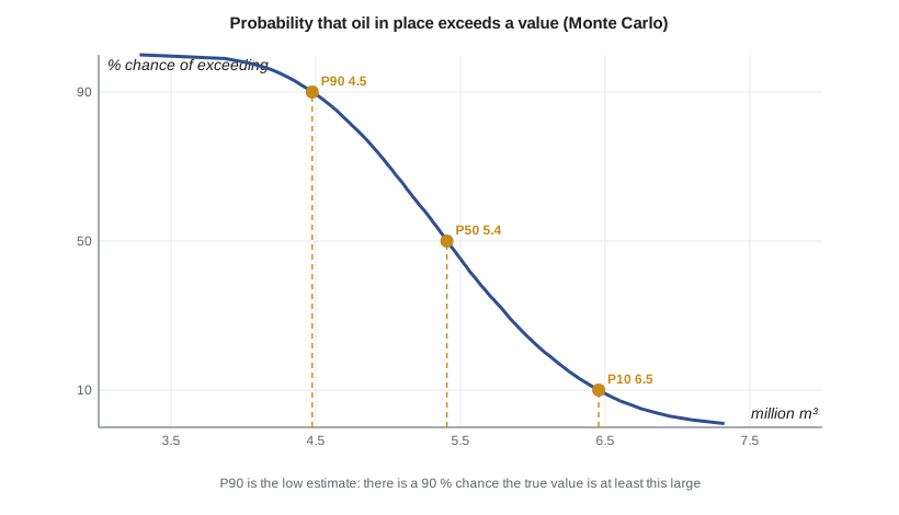
The distribution is usually shown as a cumulative exceedance curve: for each value of oil in place, the probability that the true value is at least that large. Three points are reported. P90 is the value with a 90 percent chance of being exceeded, the low estimate. P50 is the median. P10, with only a 10 percent chance of being exceeded, is the high estimate. Because the inputs multiply, the result is often skewed to the right, with the mean above the median.

The quality of a Monte Carlo result depends on the input distributions. Triangular distributions, defined by a minimum, most likely and maximum, are common because they are easy to explain. Lognormal distributions often suit thickness and permeability. Inputs that are related should be correlated in the sampling: for example, high porosity often comes with low water saturation, and ignoring that makes the range too narrow or too wide. The P90 to P10 range should be checked against experience; a range of less than about a factor of 1.3 is often a sign that the inputs are too narrow.

# Volumetric oil in place: a deterministic estimate and a Monte Carlo range (P90, P50, P10)
import random
SI = True   
random.seed(320)
if SI:   # pool area in hectares, net pay in m; oil in place in m3 of stock-tank oil
    A, h, phi, sw, boi = 1150.0, 6.5, 0.14, 0.30, 1.29
    ooip = lambda a, hh, p, s: a * 1.0e4 * hh * p * (1 - s) / boi
    ranges = {"A": (900, 1150, 1350), "h": (5.0, 6.5, 8.0)}
    unit, scale = "10^6 m3", 1.0e6
else:    # one 1,280-acre spacing unit, net pay in ft; oil in place in STB
    A, h, phi, sw, boi = 1280.0, 45.0, 0.08, 0.35, 1.456
    ooip = lambda a, hh, p, s: 7758.0 * a * hh * p * (1 - s) / boi
    ranges = {"A": (1280, 1280, 1280), "h": (38.0, 45.0, 52.0)}
    unit, scale = "MMSTB", 1.0e6
ranges["phi"] = (0.12, 0.14, 0.155) if SI else (0.065, 0.08, 0.09)
ranges["sw"] = (0.25, 0.30, 0.38) if SI else (0.30, 0.35, 0.45)
print(f"deterministic (most likely) oil in place: {ooip(A, h, phi, sw)/scale:.2f} {unit}")
tri = lambda lo, ml, hi: lo if lo == hi else random.triangular(lo, hi, ml)
trials = sorted(ooip(tri(*ranges["A"]), tri(*ranges["h"]), tri(*ranges["phi"]), tri(*ranges["sw"])) for _ in range(20000))
pct = lambda f: trials[int(f * len(trials))] / scale
mean = sum(trials) / len(trials) / scale
print(f"Monte Carlo, 20,000 trials: P90 {pct(0.10):.2f}  P50 {pct(0.50):.2f}  P10 {pct(0.90):.2f}  mean {mean:.2f} {unit}")
print("(P90 = 90 % chance the true value is at least this large)")
# Gas in place in the Birch Coulee gas pool
if SI:
    Ag, hg, pg, swg, z, T, p = 2400.0, 8.0, 0.12, 0.25, 0.88, 75 + 273.15, 21000.0
    bgi = (101.325 / p) * (T / 288.15) * z                 # reservoir m3 per standard m3
    G = Ag * 1e4 * hg * pg * (1 - swg) / bgi
    print(f"gas pool: Bgi = {bgi:.5f} rm3/sm3, OGIP = {G/1e9:.2f} x 10^9 m3 ({G*35.315/1e9:.0f} Bcf)")
else:
    Ag, hg, pg, swg, z, T, p = 6000.0, 26.0, 0.12, 0.25, 0.88, 167 + 459.67, 3050.0
    bgi = 0.02827 * z * T / p                              # reservoir ft3 per scf
    G = 43560.0 * Ag * hg * pg * (1 - swg) / bgi
    print(f"gas pool: Bgi = {bgi:.5f} ft3/scf, OGIP = {G/1e9:.0f} Bcf")

deterministic (most likely) oil in place: 5.68 10^6 m3
Monte Carlo, 20,000 trials: P90 4.48  P50 5.41  P10 6.46  mean 5.44 10^6 m3
(P90 = 90 % chance the true value is at least this large)
gas pool: Bgi = 0.00513 rm3/sm3, OGIP = 3.37 x 10^9 m3 (119 Bcf)

The deterministic estimate, with 1,150 ha of area, 6.5 m of net pay, 14 percent porosity, 30 percent water saturation and a Boi of 1.29, is 5.68 million m³ (about 35.7 million bbl). The Monte Carlo run gives P90 4.48, P50 5.41 and P10 6.46 million m³. The P50 is below the deterministic value because the water saturation range is skewed toward higher values: the most likely value is 30 percent but the maximum, near the edges of the pool, is 38 percent. Lena points out that this is typical. Mapping teams tend to quote most-likely values from the best-understood centre of a pool, while the edges are usually worse.

Recovery and the volumetric method

Volumetrics give hydrocarbons in place. To estimate recoverable volumes, the oil in place is multiplied by a recovery factor, which can come from analogous pools, from correlations, from material balance or simulation, or from decline curves once wells have produced. For gas reservoirs the volumetric method can also give recovery directly: the gas remaining at an abandonment pressure is the pore volume divided by Bg at that pressure, so recovery is 1 − Bgi/Bga for a reservoir without water influx (lesson 8).

The recovery factor carries as much uncertainty as the in-place volume, and often more. Many reserves estimates in early development are volumetric with an analog recovery factor, and they are later revised once performance data arrive. Engineers should record the source and range of every recovery factor they use.

The Birch Coulee gas pool adds a gas volume to the study. With 2,400 ha, 8 m of net pay, 12 percent porosity, 25 percent water saturation and an initial pressure of 21,000 kPa at 75 °C, Bgi is 0.00513 and the gas in place is about 3.37 billion m³ (about 119 Bcf). Lesson 8 compares this with the material balance.

Common sources of error

The largest volumetric errors usually come from the geometry: the area and the net pay. Contact depths, the edges of the pool, faults that may or may not seal, and channel sands that pinch out between wells all change the rock volume. Porosity and saturation errors matter too, especially in shaly or low-porosity rock where log interpretation is uncertain. A small systematic error in saturation, for example from a wrong Archie exponent, applies to the whole pool and does not average out.

Engineers check volumetric estimates against other evidence: the area that pressure tests and interference tests show is connected, the volumes material balance gives, and the production performance of wells. When the methods disagree, the disagreement is information. A material balance volume smaller than the volumetric one may mean parts of the pool are not connected to the wells; a larger one may mean an aquifer is supplying energy, or the pool extends beyond the map.