
PET-320 · Lesson 1 of 12 · 22 min
The reservoir engineer's job and reservoir types
Two years after the Tamarack 03-22 horizontal well came on production, Ethan Cardinal is back in the reservoir group at Prairie Crest Energy Ltd. in Calgary, working again with Lena Haugen, the senior reservoir engineer who mentored him through his first rotation. The company wants a full reservoir study of the Tamarack Lake Cardium A pool before it decides whether to drill more horizontal wells or to start a waterflood. 'Drilling built the well,' Lena says. 'Now we have to answer the questions the money depends on: how much oil is down there, how much of it we can get out, how fast, and what will help us get more. That is reservoir engineering.'
This course follows that study from the first data review to the final forecast. Each lesson adds one tool: volumetric estimates, fluid and rock properties, material balance, drive mechanisms, aquifers, gas reservoirs, well inflow, transient flow, displacement and decline curves. The last lesson puts the tools together into a recommendation. This first lesson describes what reservoir engineers do, how their work fits with the other petroleum disciplines, and how reservoirs are classified by the fluids they hold.
What reservoir engineers do
A reservoir engineer's central task is to estimate how much oil and gas a reservoir contains, how much can be recovered, and at what rate, under different development plans. Those three numbers drive almost every major decision an oil and gas company makes: how many wells to drill and where, whether to build a waterflood or a gas plant, what a property is worth when it is bought or sold, and what the company reports to its investors and regulators as reserves.
The work divides into a few connected activities. Reservoir description gathers what the geologists, geophysicists and petrophysicists know about the rock and turns it into numbers an engineer can use: area, thickness, porosity, saturation, permeability and their variation. Reservoir performance analysis studies how the reservoir has behaved so far, using pressures and production to learn things that static data cannot show, such as the size of the connected volume or the strength of an aquifer. Forecasting projects future production for each development option. Reservoir management turns the forecasts into decisions and then watches the field to check that the decisions were right.
Reservoir engineers work closely with the other disciplines. Geologists describe where the reservoir rock is and how it is arranged; petrophysicists interpret logs to give porosity and saturation; drilling and completions engineers build the wells; production engineers keep them flowing; facilities engineers design what happens at surface; and economists and reserves evaluators turn volumes into value. The reservoir engineer sits in the middle, because every plan depends on what the reservoir will do.
The tools, from simple to complex
Reservoir engineers use a ladder of methods. At the bottom are analogies: if a neighbouring pool with similar rock recovered 20 percent of its oil, this one may too. Next are volumetric calculations, which multiply rock volume by porosity and oil saturation to give oil in place, then apply a recovery factor. Material balance treats the reservoir as a tank and uses pressure and production history to estimate the oil in place and the energy driving production. Decline curve analysis fits trends to production rates and extends them. Analytical flow equations describe how fluid moves toward wells and how displacing water or gas moves through the rock. At the top are numerical reservoir simulators, which divide the reservoir into thousands or millions of cells and solve the flow equations in each.
Each method has a place. Early in a pool's life, with little data, volumetrics and analogies are all that is possible. Once production and pressure history exist, material balance and decline curves become powerful checks. Simulation is used when the decision is large and the geology complex enough to justify the effort, and it is only as good as the data and the simpler analyses that calibrate it. A good reservoir engineer uses several methods and reconciles them, rather than trusting any one.
Reservoir fluids and the phase envelope
Petroleum reservoir fluids are mixtures of hundreds of hydrocarbon compounds, from methane to heavy molecules with dozens of carbon atoms, with some nitrogen, carbon dioxide and sometimes hydrogen sulphide. Whether a mixture exists in the reservoir as liquid, gas or both depends on its composition, pressure and temperature. The previous course, PET-260, described this behaviour in detail. Here we need only the main ideas.
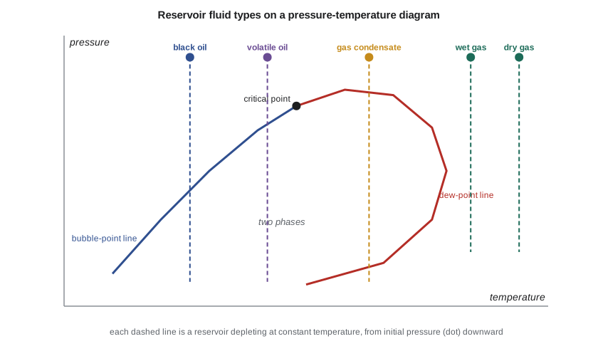
For a fixed composition, a pressure-temperature diagram shows a phase envelope. Inside it, liquid and gas coexist. Its left boundary is the bubble-point line, where the first bubble of gas appears from a liquid as pressure falls. Its right boundary is the dew-point line, where the first drop of liquid appears from a gas. The two lines meet at the critical point. Because a reservoir's temperature stays almost constant as fluids are produced, depletion is a vertical line downward on this diagram, starting at the initial pressure and temperature.
Where that line starts sets the reservoir type. If the reservoir temperature is well below the critical temperature, the fluid is an oil; as pressure falls through the bubble point, gas comes out of solution in the rock. If the temperature is between the critical temperature and the cricondentherm, the highest temperature on the envelope, the fluid is a gas condensate; as pressure falls through the dew point, liquid condenses in the rock. If the temperature is above the cricondentherm, the fluid stays gas in the reservoir throughout depletion, though a wet gas still drops liquid in the cooler surface separators while a dry gas does not.
Five fluid types in practice
Engineers usually classify fluids into five types using data easily measured at surface: the initial producing gas-oil ratio, the gravity of the stock-tank liquid and its colour. The boundaries are rules of thumb rather than physical constants, but they work well enough to choose the right analysis methods.
| Fluid type | Initial producing gas-oil ratio (approximate) | Stock-tank liquid | Reservoir behaviour |
|---|---|---|---|
| Black oil | below about 310 m³/m³ (1,750 scf/STB) | dark, usually below 45° API | gas comes out of solution below the bubble point |
| Volatile oil | about 310 to 570 m³/m³ | lighter, often above 40° API | large shrinkage; much gas released just below the bubble point |
| Gas condensate | about 570 to 2,700 m³/m³ | light coloured, above 40° API | liquid condenses in the reservoir below the dew point |
| Wet gas | about 2,700 to 18,000 m³/m³ | water-white | single-phase gas in the reservoir; liquid at surface |
| Dry gas | above about 18,000 m³/m³ | little or none | gas in reservoir and at surface |
In the Tamarack Lake field, Prairie Crest has examples of three types. The Cardium A pool is a black oil with an initial solution gas-oil ratio of about 100 m³/m³ and 38° API oil. The company's acquired light-oil pool, studied in PET-260, is also a black oil, at about 160 m³/m³. The deep Tamarack pool is a gas condensate, and the Birch Coulee gas pool, which the company bought last year, holds nearly dry gas.
Saturated and undersaturated oil reservoirs
An oil reservoir whose initial pressure is above the bubble point is undersaturated: all the gas is dissolved in the oil and there is no free gas. As it is produced, pressure falls quickly at first because liquids and rock are only slightly compressible, until the bubble point is reached. Below the bubble point, gas comes out of solution, and its expansion supplies much of the drive energy. A reservoir whose initial pressure equals the bubble point is saturated. If there is more gas than the oil can dissolve, the excess forms a gas cap above the oil, and the oil at the gas-oil contact is at its bubble point.
The Cardium A pool was discovered at about 15,300 kPa, above its bubble point of about 12,800 kPa, so it is undersaturated. Its pressure has fallen to about 14,100 kPa. Whether the pressure will drop below the bubble point, and when, is one of the questions this study must answer.
Fluid contacts and pressure gradients
Fluids in a connected reservoir separate by density: gas on top, oil in the middle and water below. The boundaries between them, the gas-oil contact and the oil-water contact, set the volume of each fluid, so they are among the most important numbers in a reservoir description. Capillary forces blur the oil-water boundary into a transition zone (lesson 4 and PET-250), so engineers distinguish the free water level, where the capillary pressure is zero, from the contact seen on logs.
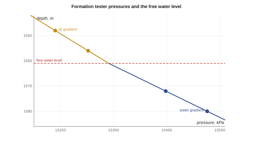
The most reliable way to find the free water level is from pressure measurements. A formation tester run on wireline or while drilling measures pore pressure at several depths. Within one fluid, pressure increases linearly with depth at that fluid's gradient: about 7.0 to 8.5 kPa/m (0.31 to 0.38 psi/ft) for light oil and 9.8 to 10.5 kPa/m (0.433 to 0.465 psi/ft) for formation water. Plotting pressure against depth and fitting a line to each fluid, the free water level is where the lines cross.
# Typing a reservoir fluid and finding the free water level from formation tester pressures
SI = True
def fluid_type(gor_scf, api):
    # Approximate field rules of thumb for initial producing gas-oil ratio (scf/STB) and stock-tank gravity
    if gor_scf < 1750 and api < 45: return "black oil"
    if gor_scf < 3200: return "volatile oil"
    if gor_scf < 15000: return "gas condensate"
    if gor_scf < 100000: return "wet gas"
    return "dry gas"
samples = [("main oil pool", 561 if SI else 794, 38 if SI else 42), ("acquired light-oil pool", 900, 40),
           ("deep Tamarack pool", 6500, 52), ("Birch Coulee gas pool", 120000, 58)]
for name, gor, api in samples:
    shown = f"{gor/5.615:,.0f} m3/m3" if SI else f"{gor:,} scf/STB"
    print(f"{name:26s} GOR {shown:>16s}  API {api}  ->  {fluid_type(gor, api)}")
# Formation tester pressures: two points in the oil leg and two in the water leg
if SI:   # depth m TVD, pressure kPa
    oil = [(1548.0, 15240.0), (1556.0, 15302.0)]
    wat = [(1572.0, 15448.0), (1580.0, 15526.0)]
    u, pu = "m", "kPa"
else:    # depth ft TVD, pressure psia
    oil = [(10400.0, 5352.0), (10430.0, 5361.6)]
    wat = [(10480.0, 5381.2), (10510.0, 5394.7)]
    u, pu = "ft", "psia"
def fit(pts):
    (z1, p1), (z2, p2) = pts
    g = (p2 - p1) / (z2 - z1); return g, p1 - g * z1
go, ao = fit(oil); gw, aw = fit(wat)
fwl = (ao - aw) / (gw - go)
print(f"oil gradient {go:.3f} {pu}/{u}, water gradient {gw:.3f} {pu}/{u}")
print(f"free water level (where the two lines cross): {fwl:,.1f} {u} TVD")main oil pool GOR 100 m3/m3 API 38 -> black oil acquired light-oil pool GOR 160 m3/m3 API 40 -> black oil deep Tamarack pool GOR 1,158 m3/m3 API 52 -> gas condensate Birch Coulee gas pool GOR 21,371 m3/m3 API 58 -> dry gas oil gradient 7.750 kPa/m, water gradient 9.750 kPa/m free water level (where the two lines cross): 1,561.0 m TVD
The formation tester points from the 102/06-14 well give an oil gradient of 7.75 kPa/m and a water gradient of 9.75 kPa/m. The lines cross at 1,561 m true vertical depth, which Ethan adopts as the free water level for the volumetric calculation in lesson 2.
Recovery factors and why they vary
The recovery factor is the fraction of the hydrocarbon in place that is eventually produced. It depends on the drive energy available, the rock and fluid properties, the well count and pattern, and the economics that set when wells are abandoned. Dry gas reservoirs often recover 70 to 90 percent of the gas in place, because gas expands so much as pressure falls. Oil reservoirs under solution-gas drive often recover only 10 to 25 percent; strong water drive or waterflooding can raise that to 35 to 50 percent or more; tight and shale oil reservoirs typically recover only a few to about 10 percent under primary production. These are wide ranges, and much of this course is about narrowing them for a particular pool.
Recovery also depends on decisions. Infill drilling, waterflooding, gas injection and better completions all change the recovery factor. That is why reservoir engineers forecast several cases: the existing wells only, more wells, and a project such as a waterflood. The difference between cases is what justifies spending money.
Reserves and resources
Volumes that are expected to be produced commercially from known accumulations under defined conditions are called reserves. In Canada, public companies report reserves under National Instrument 51-101, which requires evaluations to follow the Canadian Oil and Gas Evaluation Handbook (COGEH), prepared by qualified reserves evaluators. Proved reserves are those with a high degree of certainty, at least a 90 percent probability that the quantities recovered will equal or exceed the estimate when probabilistic methods are used. Proved plus probable reserves carry at least a 50 percent probability. Lesson 2 shows where those probabilities come from, and lesson 12 shows how decline forecasts feed reserves.
Reservoir engineers prepare the technical inputs to reserves, but reserves are a regulated, audited statement, and the classification rules are detailed. A later course, PET-450, covers them fully. For now the key idea is that every estimate in this course has uncertainty, and reserves categories are a way of describing it.
Worked problem
Classifying a fluid and estimating a contact
A new well tests at an initial producing gas-oil ratio of 420 m³/m³ with 44° API liquid. Formation tester pressures are 18,050 kPa at 1,820 m and 18,130 kPa at 1,830 m in the hydrocarbon zone, and 18,320 kPa at 1,850 m and 18,420 kPa at 1,860 m in the water zone. Classify the fluid and find the free water level.
Show solution
- 420 m³/m³ is between about 310 and 570 m³/m³, so the fluid is probably a volatile oil.
- Hydrocarbon gradient = (18,130 − 18,050)/10 = 8.0 kPa/m; water gradient = (18,420 − 18,320)/10 = 10.0 kPa/m.
- Hydrocarbon line: p = 18,050 + 8.0 (z − 1,820). Water line: p = 18,320 + 10.0 (z − 1,850).
- Setting them equal: 18,050 + 8.0z − 14,560 = 18,320 + 10.0z − 18,500, so 3,490 + 8.0z = −180 + 10.0z and z = 1,835 m.
Answer: A volatile oil; free water level about 1,835 m.
Common mistakes
MistakeTreating the oil-water contact seen on logs as the free water level.
InsteadCapillary pressure makes the log contact lie above the free water level; use pressure gradients to find the free water level.
MistakeUsing one recovery factor for every reservoir.
InsteadRecovery depends on drive mechanism, rock, fluid, well pattern and economics.
MistakeTrusting a single method.
InsteadUse volumetrics, material balance, decline curves and simulation together and reconcile them.
MistakeCalling every estimated volume a reserve.
InsteadReserves are commercial, defined-condition volumes classified by certainty under regulated rules.
Summary and key terms
- Reservoir engineers estimate hydrocarbons in place, recovery and rate, and use them to guide development decisions.
- Methods range from analogies and volumetrics to material balance, decline curves, analytical flow and numerical simulation.
- Depletion at constant temperature is a vertical line on the phase envelope; where it starts sets the fluid type.
- Black oil, volatile oil, gas condensate, wet gas and dry gas are distinguished in practice by producing gas-oil ratio and liquid gravity.
- Undersaturated oil reservoirs start above the bubble point; saturated reservoirs start at it and may have a gas cap.
- Pressure gradients from formation testers locate the free water level.
- Reserves are classified by certainty; proved, probable and possible volumes link to 90, 50 and 10 percent probabilities.
- Reservoir engineering
- The discipline that estimates hydrocarbons in place, recovery and production rates, and plans how to develop reservoirs.
- Phase envelope
- The region of pressure and temperature where liquid and gas coexist for a fixed composition.
- Bubble point
- The pressure at which the first gas comes out of solution as an oil is depressurized.
- Dew point
- The pressure at which the first liquid condenses from a gas.
- Undersaturated oil
- Oil above its bubble point, with all its gas dissolved.
- Free water level
- The depth at which capillary pressure between oil and water is zero.
- Recovery factor
- The fraction of hydrocarbon in place that is eventually produced.
- Reserves
- Volumes expected to be commercially recovered from known accumulations under defined conditions.
Practice problems
Work each problem on paper first, then reveal the answer to check.
Why is depletion drawn as a vertical line on a pressure-temperature diagram?
Show answer
Reservoir temperature stays nearly constant while pressure falls during production.
A fluid's reservoir temperature lies above its cricondentherm. Can liquid form in the reservoir?
Show answer
No. It stays gas in the reservoir, though liquid may drop out at the cooler surface conditions.
An oil gradient of 7.5 kPa/m passes through 14,000 kPa at 1,500 m; a water gradient of 9.8 kPa/m passes through 14,173 kPa at 1,520 m. Where is the free water level?
Show answer
14,000 + 7.5 (z − 1,500) = 14,173 + 9.8 (z − 1,520); solving gives 2.3z = 3,473, so z ≈ 1,510 m.
Name two decisions that depend directly on a reservoir engineer's recovery forecast.
Show answer
For example, the number and location of new wells, and whether to build a waterflood; also the value of a property and the reserves reported.
Lesson quiz · 5 questions
Score 60% or more to complete this lesson.
Create a free account to save your progress, take quizzes and earn a certificate.