Decline curve analysis and the reservoir study

The last piece of the study is the forecast. The 03-22 horizontal has two years of daily production, and the reserves evaluators want its estimated ultimate recovery before year-end. 'Decline curves are the most used tool in the business and the most abused,' Lena says. 'They are simple, which is why everyone uses them. They are empirical, which is why they go wrong. Fit them carefully, check them against what you know about the reservoir, and then pull the whole study together.'

This lesson covers Arps decline curve analysis: the exponential, hyperbolic and harmonic forms, the meaning of the decline exponent, the modified hyperbolic decline used for unconventional wells, and the estimate of ultimate recovery. It then completes the reservoir study begun in lesson 1, reconciling the volumetric, material balance and decline estimates and turning them into a recommendation.

Arps decline curves

In 1945, J. J. Arps observed that the production rate of many wells declines in a pattern that can be described by a simple equation. Define the nominal decline rate D as the fractional rate of change of production rate, D = −(1/q)(dq/dt). Arps found that D often varies with rate as D = Di (q/qi)^b, where b is the decline exponent. Integrating gives the family of curves that bears his name.

Three cases are traditionally recognized. With b = 0 the decline is exponential: D is constant and q = qi e^(−Dt). With b = 1 it is harmonic: q = qi/(1 + Di t). Between them, 0 < b < 1, it is hyperbolic. A well producing at constant flowing pressure in pseudosteady state, with constant compressibility and no change in drive, declines exponentially, so b = 0 has a physical basis (lesson 10). Values of b between 0 and 1 arise from changing drive mechanisms, such as solution-gas drive, and from layered reservoirs that deplete at different rates.

Cumulative production follows from integrating the rate. For hyperbolic decline with b not equal to 0 or 1:

For exponential decline it reduces to Np = (qi − q)/D, a useful check: the remaining reserves of a well in exponential decline are its current rate divided by its decline rate, adjusted to the economic limit.

Nominal and effective decline

Decline rates are quoted in two ways, and confusing them is a common source of error. The nominal decline D is the instantaneous rate defined above, usually per year or per month. The effective decline De is the fractional drop in rate over a period, usually one year: De = (q0 − q1)/q0. For exponential decline, De = 1 − e^(−D). For hyperbolic decline, the effective decline changes with time. Reserves reports and economic software usually specify effective annual declines, so engineers must convert carefully.

Decline exponents above one

Arps believed b would lie between 0 and 1. Multi-stage fractured horizontal wells in tight and shale reservoirs routinely fit b values of 1.2 to 2 or more over their first years. The reason is physical: these wells spend a long time in transient linear flow toward their fractures (lesson 10), for which the theory gives b = 2. Fitting such early data with a hyperbola and extending it for decades predicts far too much oil, because with b greater than 1 the cumulative production keeps growing without limit as time goes on.

The standard remedy is the modified hyperbolic decline. The well follows the fitted hyperbola until its instantaneous nominal decline falls to a terminal value Dmin, typically 5 to 10 percent per year effective, after which the forecast switches to exponential decline at Dmin. The switch represents the onset of boundary-dominated flow, when the drainage areas of neighbouring fractures and wells interfere. Reserves evaluators usually require such a terminal decline, and they check the resulting recoveries against analog wells.

Fitting decline curves well

Good decline analysis starts with clean data. Rate changes caused by operations, such as shut-ins, choke changes, artificial lift installation or offset fracturing, distort the decline and must be recognized and excluded or modelled. The fit should be made to a period when the well was producing under stable conditions with a consistent operating strategy. The decline exponent and initial decline should be consistent with the flow regime and with analog wells: a b value of 2.5 fitted to six months of data is almost certainly wrong.

Engineers increasingly use rate-transient analysis alongside decline curves. By using the flowing pressure as well as the rate, it identifies flow regimes, estimates reservoir and fracture properties and gives a physically based forecast. It is covered with well testing in PET-360. Decline curves remain the everyday tool because they need only production data, which every well has.

# Arps decline curve fit to 24 months of a horizontal well, with a terminal decline and the EUR
import math
SI = True   
if SI:   # monthly average oil rate, m3/d, Tamarack 03-22 (Cardium)
    q = [39.9, 36.9, 34.0, 30.1, 27.7, 26.6, 24.7, 24.3, 22.7, 21.3, 20.1, 19.3, 17.7, 17.3, 16.2, 16.4, 14.7, 15.1, 13.7, 13.8, 13.0, 12.6, 12.6, 11.4]
    qlim, dmin, u, vol = 1.5, 0.08, "m3/d", "m3"
else:    # monthly average oil rate, STB/d, Tamarack 3-22H (Bakken)
    q = [849, 795, 686, 599, 587, 540, 469, 449, 412, 394, 382, 350, 348, 316, 305, 308, 287, 277, 271, 259, 249, 234, 240, 238]
    qlim, dmin, u, vol = 15.0, 0.06, "STB/d", "STB"
t = [m - 0.5 for m in range(1, len(q) + 1)]                     # months
def arps(qi, D, b, tt):                                         # D: nominal monthly decline at time zero
    if b == 0: return qi * math.exp(-D * tt)
    return qi / (1 + b * D * tt) ** (1 / b)
best = None
for ib in range(0, 31):                                         # grid search on b and D; qi solved by least squares in log space
    b = ib * 0.05
    for iD in range(1, 81):
        D = iD * 0.005
        lq = [math.log(x) - math.log(arps(1.0, D, b, tt)) for x, tt in zip(q, t)]
        lqi = sum(lq) / len(lq)
        err = sum((v - lqi) ** 2 for v in lq)
        if best is None or err < best[0]: best = (err, math.exp(lqi), D, b)
err, qi, D, b = best
eff = 1 - (1 + b * D * 12) ** (-1 / b) if b else 1 - math.exp(-12 * D)
print(f"best fit: qi = {qi:.1f} {u}, initial nominal decline D = {D:.3f} per month, b = {b:.2f} (first-year effective decline {eff:.0%})")
dlim = -math.log(1 - dmin) / 12                                  # terminal nominal monthly decline from an effective annual value
cum, tt, rate, switched = 0.0, 0.0, qi, None
while rate > qlim and tt < 600:
    Dnow = D / (1 + b * D * tt)                                  # instantaneous nominal decline on the hyperbola
    if switched is None and Dnow <= dlim: switched = (tt, rate)
    if switched: rate = switched[1] * math.exp(-dlim * (tt - switched[0]))
    else: rate = arps(qi, D, b, tt)
    cum += rate * 30.4; tt += 1
print(f"switch to {dmin:.0%} per year exponential decline after {switched[0]/12:.1f} years at {switched[1]:.1f} {u}")
print(f"economic limit {qlim} {u} reached after {tt/12:.1f} years; EUR = {cum:,.0f} {vol}")
pure = sum(arps(qi, D, b, m) * 30.4 for m in range(int(tt)))
print(f"for comparison, the pure hyperbola over the same life gives {pure:,.0f} {vol} ({pure/cum - 1:+.0%})")
print(f"to date (24 months): {sum(x * 30.4 for x in q):,.0f} {vol}")

best fit: qi = 41.8 m3/d, initial nominal decline D = 0.100 per month, b = 0.90 (first-year effective decline 56%)
switch to 8% per year exponential decline after 12.4 years at 2.2 m3/d
economic limit 1.5 m3/d reached after 17.0 years; EUR = 36,266 m3
for comparison, the pure hyperbola over the same life gives 36,296 m3 (+0%)
to date (24 months): 15,264 m3

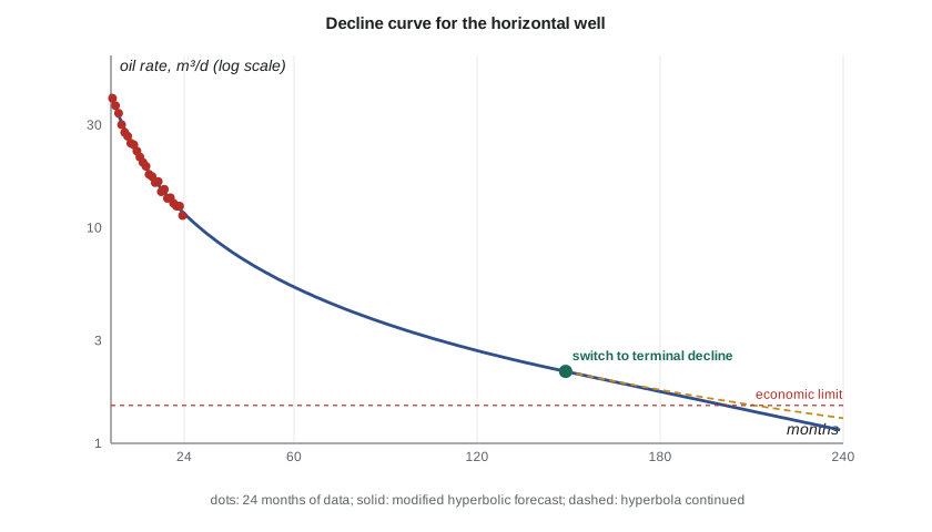
The fit to the 03-22 well's 24 months gives an initial rate of about 42 m³/d, an initial nominal decline of 0.10 per month and b = 0.9, a first-year effective decline of about 56 percent. Switching to an 8 percent per year terminal decline after about 12 years, the well reaches its 1.5 m³/d economic limit after about 17 years, with an estimated ultimate recovery of about 36,000 m³ (about 228,000 bbl), of which 15,000 m³ has been produced. Because b is below one, the terminal decline changes the answer little here.

Putting the study together

A reservoir study is not a collection of separate calculations; it is an argument in which each method checks the others. Lena asks Ethan to lay out the evidence the way the review committee will want to see it: what is in place, how it is connected, what drives it, how the wells perform, what the base case recovers, and what an investment could add.

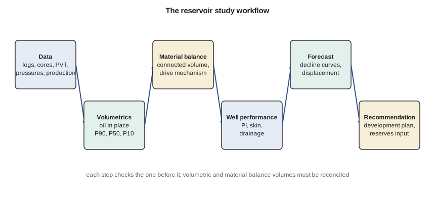
The volumetric estimate gives P90 4.48, P50 5.41 and P10 6.46 million m³ of oil in place (lesson 2). The material balance with a weak Schilthuis aquifer gives 5.11 million m³ (lessons 5 and 7), inside the volumetric range and close to its P50, so the pool is well connected and the maps are sound. The pool is undersaturated, with about 1,300 kPa above its bubble point (lessons 3 and 6), and its weak aquifer supplies a quarter of the voidage. The base case, solution-gas drive after the bubble point, recovers about 20 percent, roughly 1.0 million m³. A waterflood, started before the pressure reaches the bubble point, could raise recovery to about 33 percent, an increment of about 0.65 million m³, but the high-permeability layer seen in lesson 9 will control its sweep. The 03-22 horizontal's decline gives an estimated ultimate recovery of about 36,000 m³ per well.

The recommendation

Ethan's draft recommendation has three parts. First, start a pilot waterflood in the down-dip part of the pool within two years, before the pressure falls to the bubble point, with injection profiles monitored to manage the thief layer. Second, defer further horizontal drilling until the pilot shows how the waterflood performs, because new horizontals would accelerate the pressure decline and the gas-oil ratio rise. Third, book the decline-based reserves for the existing wells now and the waterflood volumes only when the pilot supports them. Lena adds a fourth: build the simulation model now, calibrated to this study, because the waterflood decision is large enough to justify it.

The study will be reviewed, challenged and revised. That is how reservoir engineering works: every estimate is a hypothesis to be tested by the next year of data. The methods in this course, volumetrics, material balance, flow equations, displacement and decline, are the tools for that testing, and they recur in every later petroleum course: well testing, production engineering, simulation, enhanced recovery, natural gas engineering and reserves evaluation.

Professional responsibility

Reserves and resource estimates are used by investors, lenders and governments, so the work carries professional obligations. In Alberta, engineers practise under provincial legislation administered by APEGA, and reserves disclosed by reporting issuers must be evaluated or audited by qualified reserves evaluators under National Instrument 51-101. Engineers must document their methods and assumptions, state uncertainty honestly and not let commercial pressure change a technical estimate.