Capillary pressure and transition zones

The logs from the Tamarack Lake field wells show something that puzzles Ethan. The oil-water contact is not a sharp line. Water saturation is near 100 percent at the base of the sandstone, falls steadily over the next 5 to 10 metres, and settles at about 25 percent only well above the contact. In the tighter, silty facies the change is spread over even more height. Lena explains that the reservoir is not a tank of oil floating on water but a sponge, and the sponge holds water up against gravity. 'That zone of changing saturation is the transition zone,' she says. 'It can hold a lot of oil, and if we perforate it carelessly we will produce mostly water.'

Capillary pressure in a tube

Put a thin glass tube into a beaker of water and the water rises in the tube above the level in the beaker. The water wets the glass, so the interface curves, and the curved interface has a pressure difference across it: the pressure in the non-wetting fluid above the interface is higher than in the wetting fluid below. This pressure difference is the capillary pressure, Pc, defined as the pressure in the non-wetting phase minus the pressure in the wetting phase. For a cylindrical tube of radius r it is given by the Young-Laplace equation.

Capillary pressure rises as the tube narrows, as interfacial tension rises, and as the surface becomes more strongly wetting. The water column in the tube rises until its weight balances the capillary pressure, so the height of rise is Pc divided by the density difference times gravity. Lesson 6's program showed that in a tube of 1 micrometre radius, water can be held more than 20 metres above the free water level against oil. Reservoir pores are a network of such tubes of many sizes.

The free water level and the oil-water contact

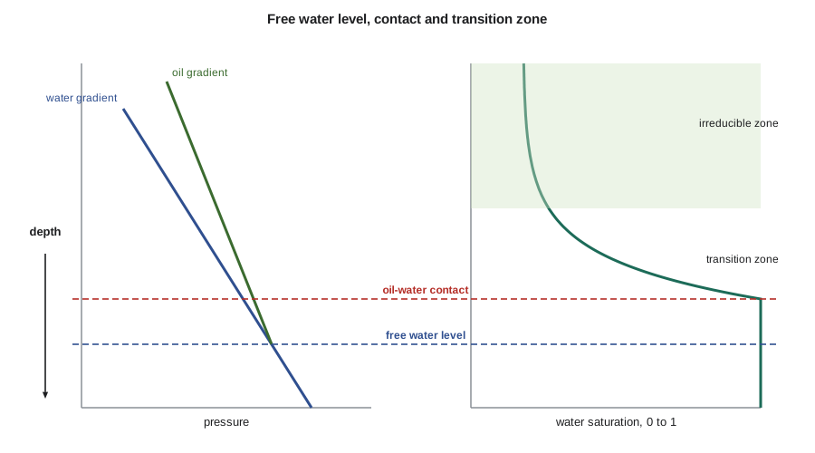
In a reservoir at equilibrium, oil and water pressures each follow their own hydrostatic gradients. The water gradient is steeper because water is denser. At some depth the two pressure lines cross: here Pc is zero, and this depth is the free water level (FWL). Above it, oil pressure exceeds water pressure by an amount that increases linearly with height. That pressure difference is the capillary pressure at that height, and it determines which pores oil can enter.

Oil enters a pore only when the capillary pressure exceeds the pore's entry pressure, which is set by its throat radius. Just above the free water level, Pc is small and oil can enter only the largest pores; higher up, oil enters progressively smaller pores, and water saturation falls toward the irreducible value. The oil-water contact (OWC) seen on logs is the depth at which oil saturation becomes measurable, which lies above the free water level by the height needed to exceed the threshold entry pressure of the largest pores. In good rock the difference may be less than a metre; in tight rock it can be many metres. Confusing the OWC with the FWL is a common source of errors in volume calculations.

Capillary pressure curves

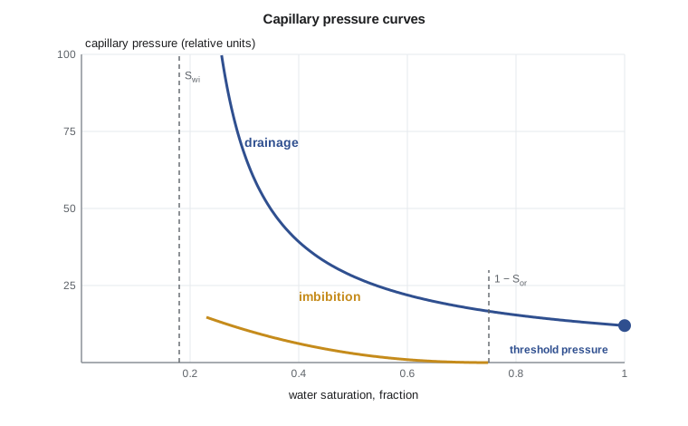
Laboratories measure how saturation changes with capillary pressure on core plugs, giving a capillary pressure curve. The drainage curve describes the non-wetting phase, oil or gas or mercury, displacing the wetting phase, water, as when oil migrated into the water-filled trap. It starts at Sw = 1, shows a threshold or entry pressure at which the non-wetting phase first enters the sample, then a plateau where most pores fill over a small pressure range, and finally rises steeply toward irreducible water saturation, where further pressure removes little more water.

The imbibition curve describes the wetting phase returning, as during a waterflood. It lies below the drainage curve, and in a water-wet rock it ends at residual oil saturation, where the oil left behind is trapped as disconnected droplets. The difference between the two curves, called capillary hysteresis, arises because pores fill and empty in different orders and because trapped oil cannot reconnect. In mixed-wet and oil-wet rocks, part of the imbibition curve has negative capillary pressure: water must be forced in.

Measuring capillary pressure

Three methods are common. In mercury injection, a clean dry plug is evacuated and mercury, which is strongly non-wetting, is forced into it at increasing pressure, up to 400 MPa (60,000 psi) in modern instruments. The volume injected at each pressure gives the saturation. It is fast and reaches very small pores, but the sample is destroyed and the fluids are not reservoir fluids. Mercury injection is also used to measure pore throat size distributions, because each pressure step corresponds to a throat radius.

In the porous plate method, a brine-saturated plug sits on a ceramic plate that lets brine but not oil or gas pass. Oil or gas pressure is applied in steps and the expelled brine measured at each step after equilibrium. It uses representative fluids and is considered the most accurate, but it can take weeks to months. In the centrifuge method, plugs are spun at increasing speeds; the centrifugal force creates a capillary pressure that varies along the plug, and the expelled fluid is measured. It is faster than the porous plate and can measure imbibition curves.

Results from mercury-air or gas-brine tests must be converted to reservoir oil-water conditions. If the pore geometry controls the curve, capillary pressure scales with σcosθ, so the reservoir curve is the laboratory curve multiplied by the ratio of σcosθ values. The ratio of mercury-air to oil-brine σcosθ is typically 10 to 15, so a mercury pressure of 100 kPa corresponds to only 7 or 8 kPa in the reservoir.

# Laboratory to reservoir capillary pressure, height above free water, and the Leverett J-function
import math
# lab mercury-air data on a plug: (Pc in kPa, wetting saturation)
lab = [(35, 1.00), (60, 0.82), (100, 0.55), (200, 0.38), (400, 0.27), (800, 0.21), (1600, 0.18)]
s_lab, cos_lab = 485.0, math.cos(math.radians(140))     # mercury-air tension mN/m and contact angle
s_res, cos_res = 26.0, math.cos(math.radians(30))        # oil-brine at reservoir conditions
conv = (s_res * cos_res) / (s_lab * abs(cos_lab))
grad = (1050 - 780) * 9.81 / 1000                        # kPa per m: water-oil density difference times g
print("  Sw    Pc res (kPa)   height above FWL (m)")
for pc, sw in lab:
    pcr = pc * conv
    print(f"{sw:5.2f} {pcr:12.2f} {pcr / grad:16.1f}")

# Leverett J lets curves from plugs of different k and phi be compared
k, phi = 46.0, 0.15                                      # mD and fraction for this plug
k_m2 = k * 0.9869e-15
for pc, sw in lab[2:5]:
    J = (pc * conv * 1000) / (s_res * 1e-3 * cos_res) * math.sqrt(k_m2 / phi)
    print(f"Sw {sw:.2f}: J = {J:.3f}")

  Sw    Pc res (kPa)   height above FWL (m)
 1.00         2.12              0.8
 0.82         3.64              1.4
 0.55         6.06              2.3
 0.38        12.12              4.6
 0.27        24.24              9.2
 0.21        48.48             18.3
 0.18        96.97             36.6
Sw 0.55: J = 0.148
Sw 0.38: J = 0.296
Sw 0.27: J = 0.592

The output shows the practical result. For this 46 mD plug, water saturation falls from 1.0 to about 0.38 within 5 metres of the free water level and to about 0.21 at 18 metres. In a reservoir only 15 metres thick, much of the oil column is in the transition zone.

The Leverett J-function

Capillary pressure curves from plugs of different permeability and porosity look different: tighter rock has smaller pores and higher capillary pressure at the same saturation. In 1941 M. C. Leverett proposed a dimensionless function that collapses curves from similar rock onto one: capillary pressure is normalized by σcosθ and multiplied by the square root of k/φ, which is proportional to a characteristic pore radius.

Once a J-function is fitted to SCAL data for a rock type, engineers can predict a capillary pressure curve, and hence saturation versus height, for any location in the model where permeability and porosity are known. This is the basis of many saturation height functions. The method works well within a single rock type but poorly across rock types with different pore geometry, so plugs are grouped first.

Pore throat size from mercury injection

Because each mercury pressure corresponds to a throat radius through the Young-Laplace equation, mercury injection curves give the distribution of pore throat sizes. Engineers use summary values from these distributions to classify rock. Winland's method, developed at Amoco and published by Kolodzie in 1980, uses the throat radius at 35 percent mercury saturation, r35, which correlates well with permeability and porosity. Rocks with r35 above about 10 micrometres are called megaporous, 2 to 10 macroporous, 0.5 to 2 mesoporous and below 0.5 microporous. Lesson 12 uses these ideas for rock typing.

In the Winland equation, r35 is in micrometres, k in millidarcies and φ in percent. It is empirical and should be checked against local mercury data, but it gives a quick way to see why two rocks with the same porosity can perform so differently.

Saturation-height functions in reservoir models

Geological and simulation models need a water saturation in every cell, and measuring it directly in each cell is impossible. Engineers therefore build saturation-height functions, equations that give water saturation as a function of height above the free water level and of rock quality. The J-function is one form: it scales capillary pressure by the square root of permeability over porosity, so a single curve can describe many rock samples. Other forms fit the log-derived saturations directly, using equations of the type Sw = a times height to the power b, with constants chosen separately for each rock type or permeability class. The function is calibrated to core capillary pressure data and checked against log saturations in wells, especially in the transition zone.

A good saturation-height function has three properties. It reproduces the log saturations in the wells used to build it. It matches the free water level found from pressure gradients. And it gives sensible saturations away from wells, where only porosity and permeability are known from the geological model. Errors in the saturation-height function feed directly into the volume of oil in place, so it deserves the same scrutiny as the porosity and net pay maps. In thick transition zones, where saturation changes over many metres, the function can change estimates of oil in place by ten percent or more.