Averaging permeability and reservoir heterogeneity

Ethan's next job sounds simple. The reservoir simulation grid for the Tamarack Lake field has blocks 100 metres on a side and 2 metres thick, and each block needs one permeability value. Each block may contain six or seven core plugs, with permeabilities ranging from 3 mD in a burrowed silty bed to 900 mD in a conglomerate stringer. Ethan averages the plugs and enters 186 mD. Lena looks at the number and asks a single question: 'Which way is the oil flowing?'

This lesson explains why there is no single correct average permeability, how to choose the right one for a given flow geometry, and how engineers measure and describe heterogeneity, the variation of permeability from place to place.

Flow along layers: the arithmetic average

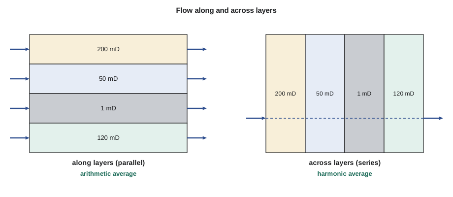
Consider a stack of horizontal layers, each with its own permeability and thickness, with fluid flowing horizontally along all of them under the same pressure gradient. Each layer carries flow in proportion to its permeability times its thickness, and the total flow is the sum. The effective permeability of the stack is therefore the thickness-weighted arithmetic average.

The arithmetic average is dominated by the best layers. In the example in the code below, one 900 mD layer that is only a tenth of the thickness carries almost half of the flow. That has a practical consequence: in a waterflood, injected water races along the high-permeability layer and reaches the producing well early, while the tighter layers are still full of oil. Knowing that the average is 186 mD is less useful than knowing that half the flow goes through one thin bed.

Flow across layers: the harmonic average

Now consider flow perpendicular to the layers, such as vertical flow through a stack of beds, or horizontal flow through blocks arranged one after another. The same flow rate must pass through every layer, and the pressure drops add. The effective permeability is the thickness-weighted harmonic average.

The harmonic average is dominated by the worst layers. A single thin bed of very low permeability can control vertical flow through a thick sandstone. In the example, a 0.5-unit bed of 3 mD drags the harmonic average down to 27 mD, a seventh of the arithmetic average. For vertical flow, a continuous shale only a few centimetres thick can act as a complete barrier, which is why geologists' maps of shale continuity matter so much for coning, gravity drainage and steam-assisted processes.

The geometric average

For a rock in which high and low permeability are scattered randomly, neither arranged in layers along the flow nor across it, theory and numerical experiments show that the effective permeability lies between the arithmetic and harmonic averages, and for a log-normal distribution in two dimensions it is close to the geometric average. The geometric average is often used as a default for randomly heterogeneous rock and for averaging plug data within a single rock type.

A useful rule: for any set of positive values, the arithmetic average is always greater than or equal to the geometric average, which is always greater than or equal to the harmonic average. The spread between them is itself a measure of heterogeneity. If all layers have the same permeability, the three averages are equal.

# Averaging permeability for layered rock, and the Dykstra-Parsons coefficient
import math, statistics
layers = [(1.0, 450.0), (2.5, 120.0), (0.5, 3.0), (3.0, 60.0), (1.0, 900.0), (2.0, 15.0)]  # (thickness, k mD)
H = sum(h for h, _ in layers)
k_arith = sum(h * k for h, k in layers) / H                 # flow along the layers
k_harm = H / sum(h / k for h, k in layers)                  # flow across the layers
k_geo = math.exp(sum(h * math.log(k) for h, k in layers) / H)
print(f"arithmetic (parallel) average {k_arith:7.1f} mD")
print(f"harmonic (series) average     {k_harm:7.1f} mD")
print(f"geometric average             {k_geo:7.1f} mD")
top = max(layers, key=lambda x: x[0] * x[1])
print(f"the {top[1]:.0f} mD layer carries {top[0] * top[1] / (k_arith * H):.0%} of the flow along the beds")

# Dykstra-Parsons coefficient from plug permeabilities (log-normal assumption)
plugs = [3, 8, 12, 15, 22, 30, 41, 55, 60, 75, 95, 120, 150, 210, 300, 450, 600, 900]
logs = sorted(math.log(k) for k in plugs)
mu, sd = statistics.mean(logs), statistics.stdev(logs)
k50 = math.exp(mu)                         # median permeability
k841 = math.exp(mu - sd)                   # value exceeded by 84.1 percent of samples
V = (k50 - k841) / k50
print(f"median {k50:.0f} mD, k at 84.1 % exceedance {k841:.0f} mD, Dykstra-Parsons V = {V:.2f}")

arithmetic (parallel) average   186.2 mD
harmonic (series) average        26.7 mD
geometric average                74.7 mD
the 900 mD layer carries 48% of the flow along the beds
median 67 mD, k at 84.1 % exceedance 14 mD, Dykstra-Parsons V = 0.79

Radial averaging around a well

Near a well, flow is radial, so annular rings of rock are in series. If permeability changes with distance from the well, for example because drilling mud damaged a ring of rock near the wellbore, the rings combine like series resistances, but each ring is weighted by the logarithm of its radius ratio instead of by its thickness. A damaged zone only a few tens of centimetres thick with a tenth of the original permeability can cut the well's productivity in half. Engineers express such near-well effects as a skin factor, which the later well testing course treats in detail.

Measuring heterogeneity

Engineers use several numbers to describe how heterogeneous a reservoir is. The simplest is the ratio of the arithmetic to the harmonic average. The most widely used in waterflood studies is the Dykstra-Parsons coefficient, V, introduced in 1950 for predicting how evenly water sweeps through a layered reservoir.

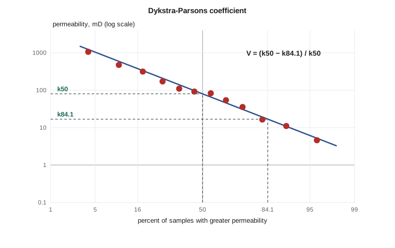
To find V, the permeabilities of all samples in an interval are sorted and plotted on log-probability paper: the logarithm of permeability against the percentage of samples with a higher permeability. If permeability is log-normally distributed, the points fall on a straight line. V is calculated from the median permeability, k₅₀, and the permeability exceeded by 84.1 percent of samples, which is one standard deviation below the median on the log scale.

V ranges from 0 for a perfectly uniform reservoir to 1 for an infinitely heterogeneous one. Most sandstone reservoirs have V between 0.5 and 0.9. A value near 0.5 indicates a reasonably uniform reservoir in which a waterflood sweeps the layers fairly evenly; a value above about 0.8 indicates strong layering in which water will channel through the best layers and leave much oil behind unless the flood is managed with profile control, selective completions or polymer.

The Lorenz coefficient is another heterogeneity measure. Layers are sorted from highest to lowest permeability-to-porosity ratio, and cumulative flow capacity, the fraction of total kh, is plotted against cumulative storage capacity, the fraction of total φh. A homogeneous reservoir plots on the diagonal; a heterogeneous one bows above it, because a small fraction of the pore volume carries a large fraction of the flow. The Lorenz coefficient is the area between the curve and the diagonal, doubled, and ranges from 0 to 1. Its plot is easy to read: if 20 percent of the storage carries 70 percent of the flow, the flood will be dominated by a few layers.

Heterogeneity at every scale

Heterogeneity exists at every scale, and different processes create it. At the millimetre scale, laminae of different grain size give a single plug anisotropy. At the bed scale, shale drapes and cemented layers interrupt vertical flow. At the field scale, the Cardium shoreface sandstones thin and shale out landward, and conglomerates occur only in patchy lenses. Faults break the reservoir into blocks with different pressures and contacts. Each scale must be represented somehow in the model, either explicitly in the grid or through effective properties.

Upscaling is the general name for computing effective block properties from finer-scale data. Simple averages work for simple geometries. For complex ones, engineers run small flow simulations on a fine grid representing one coarse block and compute the permeability that gives the same flow, a process called flow-based upscaling. Whatever the method, the important point is that permeability averages depend on geometry and flow direction, and no single number captures a heterogeneous rock.

Spatial correlation

Heterogeneity is not just about the range of values but about how they are arranged. A reservoir with high-permeability layers that are continuous between wells behaves very differently from one where the same values occur in short, isolated lenses, even if the histograms are identical. Geostatistics describes this arrangement using the variogram, which measures how different two values become as the distance between them increases. The distance at which values stop being related is the correlation length or range. Geologists estimate it from outcrop studies, closely spaced wells and depositional models, because most wells are too far apart to measure it directly. Geostatistical methods then generate many equally probable maps of permeability that match the well data and the variogram, and engineers run simulations on several of them to see how much the uncertainty in arrangement affects recovery.

Upscaling for simulation models

A geological model may contain tens of millions of cells a few metres across, each with a porosity and permeability drawn from logs and core. A reservoir simulator usually cannot run that many cells fast enough for the dozens or hundreds of cases an engineer needs, so the fine model is upscaled into coarser cells. Porosity upscales simply: the pore volume of the coarse cell is the sum of the pore volumes of the fine cells, so a bulk-volume-weighted arithmetic average is exact. Permeability is harder because, as this lesson has shown, the right average depends on the direction of flow and on how the fine cells are arranged. Simple upscaling uses the arithmetic average of the fine cells for horizontal permeability and the harmonic average for vertical permeability. Flow-based upscaling instead solves a small single-phase flow problem across each coarse cell with pressure boundaries applied on opposite faces and finds the permeability that gives the same flow rate. Flow-based methods capture the connectivity of high- and low-permeability streaks that simple averages miss.

Upscaling always loses information. Thin, continuous shales that stop vertical flow, or thin high-permeability streaks that carry injected water quickly to producers, can vanish if the coarse cells are too thick. A good practice is to compare a fine-grid and a coarse-grid simulation of a representative sector before relying on the coarse model, and to keep layer boundaries at major flow barriers.