Basin analysis and the petroleum system events chart

Ten weeks into the study, Nadia's team has maps of reservoirs, source rocks, seals and traps across the area. What it lacks is time. The dome west of the Tamarack Lake field formed when the Leduc reef grew in the Late Devonian, and the Duvernay shale beside it generated oil much later, when the basin was buried beneath the sediments shed from the rising Rockies. 'Every element can be present and the well can still be dry if they happened in the wrong order,' Nadia says. 'Now we put it all on one clock.' Basin analysis reconstructs the history of a basin to test whether its petroleum systems worked, and the events chart is its most compact summary.

The petroleum system concept

Leslie Magoon and Wallace Dow formalized the petroleum system concept in the 1990s. A petroleum system includes a pod of active source rock and all the oil and gas that came from it, together with the geological elements and processes needed for accumulations to exist: source, reservoir, seal and overburden rocks, and the processes of trap formation and of generation, migration and accumulation. Each system is named after its source rock and its main reservoir, with a symbol indicating the level of certainty: known (!) when oil has been geochemically matched to its source, hypothetical (.) when the source is identified but not matched, and speculative (?) when both are inferred.

The concept separates the system, which exists in nature, from the play and the prospect, which are exploration ideas. A system may contain many plays; a play may contain many prospects. Thinking in systems encourages geologists to account for all the petroleum a source rock generated, not just the fields already found, and to ask where the rest went. Comparing the volume generated with the volume discovered gives the system's efficiency, often only a few percent for conventional accumulations, and highlights how much may remain, either undiscovered or still in the source rock.

Reconstructing burial and heat

The backbone of basin analysis is the burial history, a plot of depth against time for each layer. It is built by backstripping: starting from the present stratigraphy in a well or pseudo-well, the geologist removes layers one by one from the top, decompacting the remaining layers with the compaction laws of Lesson 1, and restoring any thickness eroded at unconformities. Each step shows where the layers were at an earlier time. The result shows when the basin subsided rapidly, when it paused, and when it was uplifted and eroded.

Heat flow comes next. Temperature at depth depends on the heat flowing up from the Earth's interior, the thermal conductivity of the rocks, and heat generated by radioactive decay in the crust. Present-day temperatures are measured in wells, though the readings must be corrected because drilling mud cools the borehole. Past temperatures are inferred from maturity indicators such as vitrinite reflectance and from the tectonic history: rifting raises heat flow, and thick sediment piles insulate the layers below. Calibrating the model so that it reproduces the measured temperatures and maturities in wells is the main test of a basin model.

With burial and temperature histories in hand, the model calculates the maturity of each source rock through time, using chemical kinetic models that describe how kerogen breaks down into oil and gas, as Lesson 5 introduced with the simpler TTI method. Modern basin modelling software extends this to two and three dimensions, simulating pressure, the expulsion and migration of oil and gas, and their accumulation in traps. These models are uncertain, but they make assumptions explicit and allow alternative scenarios to be compared.

The events chart

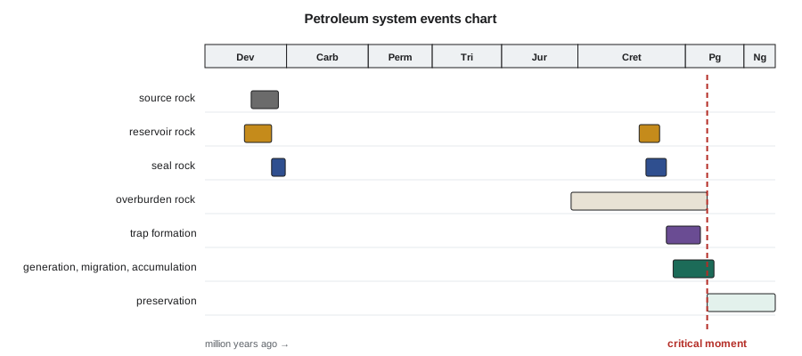
The events chart summarizes a petroleum system on a single timeline. Horizontal bars show when each element was deposited: source rock, reservoir, seal, overburden. Further bars show when traps formed and when the source rock generated, expelled and migrated petroleum. A vertical line marks the critical moment, the time when most of the petroleum in the system was generated and migrating. After it comes the preservation time, during which accumulations must survive uplift, erosion, fault leakage and biodegradation. The chart makes the essential question obvious: did the traps exist before the critical moment, and have they survived since?

The events chart also guides exploration strategy. If traps formed late, after the critical moment, only those that could have received oil remigrated from earlier accumulations or still-generating source rock are prospective. If the critical moment was long ago and the basin has since been uplifted, preservation is the main risk. If the source is still in the oil window today, recently formed traps may be charged. Different petroleum systems in the same basin can have very different charts.

# Timing check: when does the source rock enter and peak in the oil window, compared with trap formation?
T_SURFACE = 10.0
START, STEP = 380.0, 0.5            # source rock deposited 380 Ma; time step in million years

def depth_km(age):
    # burial history: slow Paleozoic burial, pause, rapid foreland burial 100-55 Ma, then 1.5 km of uplift
    if age > 250: return 1.2 * (START - age) / (START - 250)
    if age > 100: return 1.2 + 0.3 * (250 - age) / 150
    if age > 55:  return 1.5 + 2.6 * (100 - age) / 45
    return 4.1 - 1.5 * (55 - age) / 55

def history(gradient):
    tti, onset, peak, end = 0.0, None, None, None
    age = START
    while age > 0:
        T = T_SURFACE + gradient * depth_km(age - STEP / 2)
        tti += STEP * 2.0 ** int((T - 100) // 10)
        if onset is None and tti >= 15: onset = age
        if peak is None and tti >= 75: peak = age
        if end is None and tti >= 160: end = age
        age -= STEP
    return tti, onset, peak, end

traps = {"Devonian reef buildup": 370, "fold above reactivated fault": 70, "late fault trap": 30}
for g in (26, 30):
    tti, onset, peak, end = history(g)
    fmt = lambda a: f"{a:.0f} Ma" if a else "not reached"
    print(f"gradient {g} C/km: oil generation begins {fmt(onset)}, peaks {fmt(peak)}, ends {fmt(end)}; TTI today {tti:.0f}")
    for name, formed in traps.items():
        if onset is None: verdict = "no charge: source immature"
        elif formed >= onset: verdict = "formed before generation began: can receive the full charge"
        elif peak is None or formed > peak: verdict = "formed during early generation: partial charge"
        else: verdict = "formed after peak generation: little charge unless oil remigrates"
        print(f"   {name:30s} formed {formed} Ma -> {verdict}")

gradient 26 C/km: oil generation begins 60 Ma, peaks not reached, ends not reached; TTI today 69
   Devonian reef buildup          formed 370 Ma -> formed before generation began: can receive the full charge
   fold above reactivated fault   formed 70 Ma -> formed before generation began: can receive the full charge
   late fault trap                formed 30 Ma -> formed during early generation: partial charge
gradient 30 C/km: oil generation begins 70 Ma, peaks 54 Ma, ends 30 Ma; TTI today 185
   Devonian reef buildup          formed 370 Ma -> formed before generation began: can receive the full charge
   fold above reactivated fault   formed 70 Ma -> formed before generation began: can receive the full charge
   late fault trap                formed 30 Ma -> formed after peak generation: little charge unless oil remigrates

The program reuses the time-temperature approach of Lesson 5 to find when generation began and peaked, then compares those ages with the times at which three traps formed. A trap that formed after the peak can still be charged if generation continued, but it receives less oil. The program also shows how sensitive the conclusion is to the heat flow assumption, which is why modellers present several scenarios.

Pressure and its history

Basin analysis also reconstructs fluid pressure. In many basins, pressure below a certain depth rises faster than the hydrostatic gradient, a condition called overpressure. It develops where fine-grained sediments are buried too fast for their water to escape, so the water carries part of the weight of the overlying rock, and where oil and gas generation adds fluid volume in tight source rocks. Overpressure matters to geologists because it slows compaction and preserves porosity, drives primary migration and can fracture seals; it matters to drilling engineers because unexpected pressure causes kicks and blowouts. Tight-oil plays such as the Montney, the Duvernay, the Bakken and the Wolfcamp are commonly overpressured in their best areas, and that extra pressure is part of why wells there produce strongly. Uplift and erosion can do the opposite, leaving some reservoirs underpressured, a condition that is common in parts of western Canada and the Rocky Mountain basins and that affects how wells must be drilled and produced.

Play fairways and common risk segment maps

To move from a basin model to exploration decisions, geologists map play fairways, the areas where all the elements of a play are likely to be present. Each element is mapped separately as a risk map: where the reservoir is likely to be present and of good quality, where the seal is effective, where the source rock is mature and on a migration route. Overlaying the maps, often colour-coded green, yellow and red for low, moderate and high risk, produces a common risk segment map that shows where the play is most likely to work. Prospects inside the green areas share less risk than those in red areas.

Prospect risk is usually expressed as a probability of geological success, the chance that a well will find a flowing accumulation of a given minimum size. It is estimated as the product of the probabilities of each independent element: source and charge, reservoir, trap and seal, and timing and preservation. Because the probabilities multiply, a prospect with four elements each at 0.7 has a chance of success of only 0.24. Volumes are estimated as ranges, commonly reported as P90, P50 and P10 values, where P90 is a low case exceeded with 90 percent probability and P10 a high case exceeded with only 10 percent probability.

Learning from results

Exploration is a learning process. Every well, successful or not, tests the assumptions behind the basin model and the risk maps. A dry hole may show that the reservoir was absent, the seal leaked, or the trap was never charged; each answer changes the risk on neighbouring prospects. Look-backs, systematic comparisons of predicted and actual results across many wells, show whether a team's probabilities are calibrated: if prospects risked at 30 percent succeed only 10 percent of the time, the team has been too optimistic. Companies that review their predictions honestly tend to make better decisions over time.

The Western Canada Sedimentary Basin shows the value of this learning. Exploration began with structural traps in the foothills, moved to the Devonian reefs after Leduc in 1947, then to Cretaceous stratigraphic traps, and most recently to the source rocks themselves in the Montney and Duvernay plays. Each step was made possible by better understanding of the basin's petroleum systems, and each opened large new volumes in a basin that had been called mature several times.