Seismic interpretation for petroleum geologists

The dome west of the Tamarack Lake field exists so far only on a single old two-dimensional seismic line. Before Prairie Crest spends millions on a well, Nadia wants to know whether it is real, how big it is, and whether the Leduc reef she suspects inside it can be seen on the data. She licenses a three-dimensional survey that covers the area and sits Ethan at a workstation beside her. 'Seismic is the only tool that shows us the rocks between the wells,' she says. 'But it shows them in time, not depth, and through a blurry lens. Interpretation is learning to see through the lens.' PET-200 explained how seismic data are acquired; this lesson is about reading them.

What a seismic section shows

A seismic section is a picture of echoes. Sound waves sent into the ground reflect wherever the acoustic impedance, the product of rock density and sound velocity, changes. The strength and polarity of each reflection depend on the reflection coefficient, the difference in impedance across the boundary divided by the sum. A boundary where a fast, dense limestone overlies a slow shale gives a strong reflection of one polarity; a gas sand beneath shale, slower and less dense, gives a strong reflection of the opposite polarity. The section plots these reflections against two-way travel time, the time for sound to go down to a reflector and back, in milliseconds.

The seismic trace at any location is approximately the series of reflection coefficients at each boundary, smeared by the seismic wavelet, the short pulse of sound that was sent and returned. This smearing, called convolution, means thin layers produce overlapping wavelets that interfere. Layers thinner than about one quarter of the dominant wavelength, often 10 to 30 metres in the depth range of many reservoirs, cannot be resolved as separate top and base reflections, though their presence still changes the amplitude. Below about one thirtieth of a wavelength, they are effectively invisible.

Tying wells to seismic

The first step in any interpretation is the well tie, which links reflections to rock layers. Using the sonic and density logs from a well, the interpreter calculates the impedance at every depth, then the reflection coefficients, and convolves them with a wavelet estimated from the seismic data. The result, a synthetic seismogram, should look like the seismic trace at the well location. Matching the two, and adjusting the time-depth relationship from a checkshot or vertical seismic profile, tells the interpreter which reflection is the top of the reservoir, which is the base of the seal, and so on. Without a good tie, every horizon picked afterward may be the wrong rock.

Several measurements support the tie. A checkshot survey records the time for sound from a surface source to reach geophones placed at known depths in the well, giving a direct time-depth curve. A vertical seismic profile records the full waveform at many depths and shows exactly how the seismic wavelet changes as it travels down. Sonic logs alone tend to give slightly faster velocities than the surface seismic, because they measure at higher frequencies over a short distance, so they are adjusted, or drift-corrected, to match the checkshots. The tie also confirms the polarity of the data, which convention the processors used for a positive reflection, without which the interpreter could pick a trough when the reservoir top is a peak.

# Two-way time to depth through layered interval velocities, and depth sensitivity to velocity error
# layers: (name, two-way time at base in ms, interval velocity in m/s)
layers = [("Tertiary and Upper Cretaceous", 520, 2300), ("Cretaceous shales and sands", 1100, 2900),
          ("Jurassic to Mississippian", 1500, 3600), ("Upper Devonian shales", 1795, 3900)]

depth, t_prev = 0.0, 0
print("layer                          base TWT (ms)   thickness (m)   base depth (m)")
for name, t, v in layers:
    dz = v * (t - t_prev) / 1000 / 2
    depth += dz; t_prev = t
    print(f"{name:30s} {t:8d}       {dz:10.0f}      {depth:10.0f}")
v_avg = depth / (t_prev / 1000 / 2)
print(f"\naverage velocity to the target: {v_avg:,.0f} m/s")
for err in (-0.02, -0.01, 0.01, 0.02):
    print(f"velocity error {err:+.0%} -> depth {depth * (1 + err):6.0f} m ({depth * err:+.0f} m)")

layer                          base TWT (ms)   thickness (m)   base depth (m)
Tertiary and Upper Cretaceous       520              598             598
Cretaceous shales and sands        1100              841            1439
Jurassic to Mississippian          1500              720            2159
Upper Devonian shales              1795              575            2734

average velocity to the target: 3,047 m/s
velocity error -2% -> depth   2680 m (-55 m)
velocity error -1% -> depth   2707 m (-27 m)
velocity error +1% -> depth   2762 m (+27 m)
velocity error +2% -> depth   2789 m (+55 m)

The program converts the two-way time of the target horizon to depth using a layered velocity model and then shows how a small error in velocity changes the depth. A 2 percent error in average velocity moves a reflector at about 2,700 metres by roughly 55 metres, comparable to the closure of many traps. This is why depth conversion is one of the largest uncertainties in mapping a structure, and why interpreters calibrate velocities carefully with every well.

Picking horizons and faults

Interpretation proceeds by picking horizons, continuous reflections that represent the same geological surface, across the survey, and faults, where reflections are offset. In three-dimensional data, interpreters work on vertical sections in several directions and on horizontal time slices, which show the layers in map view. Software can track a horizon automatically along a consistent peak or trough, but faults, poor data and changes in the character of the reflection require judgment. Faults appear as lines of offset reflections, sometimes with a change in dip or a loss of continuity; mapping them in three dimensions reveals their throw, their linkage and which blocks they isolate.

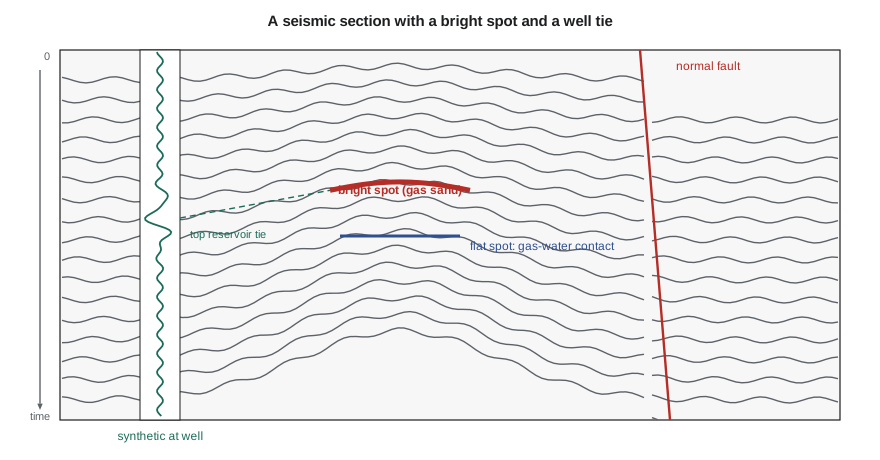
Interpreters also look at the geometry of reflections within packages, a method called seismic stratigraphy that underlies the sequence stratigraphy of Lesson 8. Reflections that end against a surface above (toplap) or below (onlap, downlap), or are cut off by it (truncation), mark sequence boundaries and flooding surfaces. Sloping clinoforms show where shelves built out into deeper water. Mounded reflections can indicate reefs or fans; chaotic reflections can indicate slumps, karst or salt. Reading these patterns lets geologists map depositional environments before any well is drilled.

Seismic attributes and direct hydrocarbon indicators

Beyond structure, seismic data carry information about the rocks and fluids themselves. A seismic attribute is any quantity derived from the data: amplitude, frequency, phase, coherence, curvature and many more. Amplitude maps of a horizon can show where a sand is thick or thin, or where porosity changes. Coherence and curvature highlight faults and fractures. Spectral decomposition, which separates the data into frequency bands, reveals thin channels that cannot be seen at the full bandwidth. Time slices and horizon slices through a three-dimensional survey can show ancient river channels and deepwater fans in astonishing detail.

Under some conditions, hydrocarbons themselves change the seismic response, producing direct hydrocarbon indicators. Gas, even in small amounts, greatly lowers the velocity of a porous rock. In young, soft sandstones such as those of the Gulf of Mexico, this creates bright spots, unusually strong reflections at the top of gas sands, and flat spots, horizontal reflections at the gas-water or oil-water contact that cut across the dipping layers. Amplitude versus offset (AVO) analysis compares how reflection strength changes with the angle at which sound hits the boundary; gas sands often show amplitudes that grow with offset. These techniques revolutionized deepwater exploration from the 1970s onward, but they can mislead: low-saturation gas, called fizz gas, can produce bright spots without commercial volumes, and in hard, older rocks fluid effects are small.

Seismic inversion converts reflection data back into estimates of impedance and, with enough angle information, other elastic properties layer by layer. Combined with well logs and rock physics models, which relate elastic properties to porosity, lithology and fluid, inversion can produce maps of porosity or of brittleness for tight-oil and shale plays. Repeated surveys over a producing field, called time-lapse or 4D seismic, show how fluids move as oil is produced and water or gas replaces it, helping engineers place infill wells.

Seismic in tight-oil and shale plays

Seismic interpretation is not only for finding traps. In tight-oil and shale plays, where the oil is spread through a continuous layer, three-dimensional seismic helps engineers avoid hazards and find the best rock. Small faults that cut the target can divert hydraulic fractures or connect them to water-bearing layers, so they are mapped with coherence and curvature attributes before wells are planned. Thickness maps from the seismic guide the landing depth. Inversion for elastic properties can highlight more brittle zones that fracture well. In parts of Alberta, the Montney and Duvernay plays have also required seismic mapping of faults to manage the risk of induced earthquakes from hydraulic fracturing, as PET-200 described.

An interpretation workflow

A typical interpretation project follows a sequence. The interpreter first checks the data: survey geometry, processing history, polarity and phase. Next come the well ties and a first time-depth model. Key horizons, usually a few strong, regionally continuous reflections, are picked on a coarse grid of lines and checked around loops, then tracked across the whole survey. Faults are interpreted and connected into a fault framework. Time maps are converted to depth with a velocity model calibrated to the wells, and the depth maps are compared with well tops; any misfit at a well indicates a velocity or picking error to be fixed. Finally, attributes and inversion are used to map reservoir properties, and the results are handed to the geological modellers and engineers with a clear statement of uncertainty.

Pitfalls

Seismic interpretation is full of traps for the unwary, called pitfalls. Velocity pull-ups and push-downs make reflections beneath fast or slow bodies, such as reefs, salt, gas clouds or shallow channels, appear higher or lower in time than they are, creating false structures or hiding real ones. Multiples, sound that bounced more than once between strong reflectors, can mimic real layers. Migration, the processing step that moves reflections to their true positions, may be imperfect near steep dips and salt. Faults may be mis-correlated across, linking the wrong horizons. Every interpreted horizon is a hypothesis, and the best interpreters keep asking which observations could prove it wrong.

In Western Canada, pull-ups are a classic issue over Devonian reefs: the reef limestone is faster than the surrounding shale, so overlying reflections rise in time over the reef even where there is no structure. Early explorers used this to find reefs on seismic data, while also learning not to mistake the pull-up for a structural closure in the shallower section.