Robot kinematics: forward kinematics

Robot R1 arrives at Baywind's shop in its crate in week eleven, and Simone invites Owen and Gilles to watch it being commissioned. The robot is a six-axis articulated arm of the 20 kg payload class, the most common type of industrial robot in the world. Its six revolute joints, from the base outward, rotate the whole arm about a vertical axis, swing the upper arm, swing the forearm, roll the forearm, bend the wrist and turn the flange. Before Owen can check any robot program he must be able to answer a basic question: given the six joint angles, where is the gripper, and which way is it pointing? That question is forward kinematics. This lesson, and the next on the reverse question, cover the mechanical engineer's core of robotics. The robotics programme's kinematics course (ROB-210) treats the same material at greater depth, including quaternions and screw theory; here the aim is to read and check an industrial robot's geometry with confidence.

Positions and orientations

A rigid body in space has six degrees of freedom: three of position and three of orientation. Robots describe both with coordinate frames. A frame is an origin and three perpendicular unit axes. The robot's base frame sits at its foot; the tool frame, at the tool centre point (TCP), sits at the working point of the gripper with its z axis usually pointing out of the tool. The pose of the tool is the position and orientation of the tool frame relative to the base frame.

Orientation is described by a 3 × 3 rotation matrix whose columns are the tool frame's x, y and z axes expressed in base coordinates. A rotation matrix is orthonormal: its columns are unit vectors perpendicular to each other, so its transpose is its inverse and its determinant is +1. Robot controllers display orientation more compactly, as three angles (roll, pitch and yaw, or one of several Euler angle conventions) or as a four-number unit quaternion, but internally all of them are equivalent to the matrix. The conventions differ between robot makers, which is a frequent source of confusion when programs or offline simulations move between systems.

Homogeneous transforms

Position and orientation are combined in a 4 × 4 homogeneous transformation matrix:

where R is the rotation matrix and p the position of the frame's origin. A point with coordinates in the tool frame, written as a four-vector with a final 1, is converted to base coordinates by multiplying by T. The great convenience is that transforms chain by multiplication: if \(T_{01}\) gives frame 1 relative to frame 0 and \(T_{12}\) gives frame 2 relative to frame 1, then \(T_{02} = T_{01} T_{12}\). A serial robot is a chain of links, each moving relative to the one before, so its forward kinematics is a product of six link transforms followed by the fixed tool transform.

Denavit-Hartenberg parameters

Each link transform depends on the joint angle and on fixed dimensions of the link. The Denavit-Hartenberg (DH) convention, introduced in 1955, describes each link with just four numbers by placing the frames carefully: the z axis of each frame lies along a joint axis, and the x axis lies along the common perpendicular between successive joint axes. The four parameters are then the joint angle \(\theta\) about z, an offset d along z, a length a along x, and a twist \(\alpha\) about x. In the standard form each link's transform is

and the robot's forward kinematics is \(T = A_1 A_2 A_3 A_4 A_5 A_6 T_{tool}\). A modified DH convention, which places each frame at the start rather than the end of its link, is common in textbooks and some software, and gives different numbers for the same robot. Robot makers often publish dimensions rather than DH tables, and their controllers use their own internal conventions, so the first step in any kinematic check is to settle which convention a table uses.

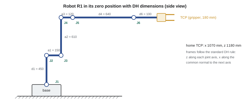
The DH table for R1, built from the dimensions in the figure, is in the program below. The values are illustrative of robots of this class rather than any one model. The second joint has an offset of −90° so that the upper arm points straight up when its joint reads zero, which matches how robot makers usually define the zero position. The gripper's TCP is 180 mm beyond the flange along the flange's z axis.

# Forward kinematics of robot R1 with Denavit-Hartenberg (DH) parameters
import math
def dh(theta, d, a, alpha):
    ct, st, ca, sa = math.cos(theta), math.sin(theta), math.cos(alpha), math.sin(alpha)
    return [[ct, -st * ca, st * sa, a * ct], [st, ct * ca, -ct * sa, a * st], [0, sa, ca, d], [0, 0, 0, 1]]
def mul(A, B):
    return [[sum(A[i][k] * B[k][j] for k in range(4)) for j in range(4)] for i in range(4)]

# Standard DH table for a typical six-axis industrial arm (illustrative dimensions, metres and radians)
#        d       a       alpha        joint offset
DH = [(0.450, 0.150, -math.pi / 2, 0.0),
      (0.000, 0.610,  0.0,         -math.pi / 2),
      (0.000, 0.120, -math.pi / 2, 0.0),
      (0.640, 0.000,  math.pi / 2, 0.0),
      (0.000, 0.000, -math.pi / 2, 0.0),
      (0.100, 0.000,  0.0,         0.0)]
tool = [[1, 0, 0, 0], [0, 1, 0, 0], [0, 0, 1, 0.180], [0, 0, 0, 1]]   # gripper TCP 180 mm along flange z

def fk(q_deg, with_tool=True):
    T = [[1, 0, 0, 0], [0, 1, 0, 0], [0, 0, 1, 0], [0, 0, 0, 1]]
    for (d, a, al, off), q in zip(DH, q_deg):
        T = mul(T, dh(math.radians(q) + off, d, a, al))
    return mul(T, tool) if with_tool else T

c = lambda v: f"{round(v, 3) + 0.0:+.3f}".replace('-0.000', '+0.000')

def show(name, q):
    T = fk(q)
    x, y, z = (T[i][3] * 1000 for i in range(3))
    print(f"{name:26s} q = {q}  ->  TCP x {x:7.1f}  y {y:7.1f}  z {z:7.1f} mm, tool z-axis ({c(T[0][2])}, {c(T[1][2])}, {c(T[2][2])})")
    return T

show("home (all joints zero)", [0, 0, 0, 0, 0, 0])
show("over the infeed pallet", [35, 20, 10, 0, 60, 35])
show("at the balancing arbor", [-50, 35, -5, 0, 60, -50])
T = fk([35, 20, 10, 0, 60, 35]); R = [row[:3] for row in T[:3]]
ortho = max(abs(sum(R[k][i] * R[k][j] for k in range(3)) - (1 if i == j else 0)) for i in range(3) for j in range(3))
print(f"Check: rotation part is orthonormal to within {ortho:.1e}")
# Sensitivity: a 0.01 degree error in joint 2 moves the TCP by about
T1, T2 = fk([35, 20, 10, 0, 60, 35]), fk([35, 20.01, 10, 0, 60, 35])
print(f"0.01 degree in joint 2 moves the TCP {1000*math.dist([T1[i][3] for i in range(3)], [T2[i][3] for i in range(3)]):.3f} mm")

home (all joints zero)     q = [0, 0, 0, 0, 0, 0]  ->  TCP x  1070.0  y     0.0  z  1180.0 mm, tool z-axis (+1.000, +0.000, +0.000)
over the infeed pallet     q = [35, 20, 10, 0, 60, 35]  ->  TCP x   796.9  y   558.0  z   527.1 mm, tool z-axis (+0.000, +0.000, -1.000)
at the balancing arbor     q = [-50, 35, -5, 0, 60, -50]  ->  TCP x   716.2  y  -853.5  z   453.6 mm, tool z-axis (+0.000, +0.000, -1.000)
Check: rotation part is orthonormal to within 4.4e-16
0.01 degree in joint 2 moves the TCP 0.144 mm

Checking the result

Forward kinematics is easy to program and easy to get wrong, so every implementation needs checks. The first is the zero position, where the answer can be read from the drawing: with all joints at zero, the TCP should lie straight out along x at \(a_1 + d_4 + d_6 + 180 = 1{,}070\) mm and at a height of \(d_1 + a_2 + a_3 = 1{,}180\) mm. The program agrees, and it shows the tool's z axis pointing along +x, horizontally forward. The second is that the rotation part remains orthonormal after six multiplications; it does, to 4 × 10⁻¹⁶, which is rounding. The third check is against the robot itself: jog it to a set of joint angles and compare the TCP position its controller reports, or better, the position measured with a laser tracker, with the calculation.

The two working poses show something useful. Over the infeed pallet, with joints (35°, 20°, 10°, 0°, 60°, 35°), the TCP is at (796.9, 558.0, 527.1) mm and the tool points straight down. At the balancing arbor, with joint 1 at −50°, the TCP is at (716.2, −853.5, 453.6) mm, again pointing down. In both, the wrist angle of 60° plus the shoulder and elbow angles of 30° total 90°, which tilts the tool vertical: a pattern worth recognizing when reading robot programs. The final lines show how a tiny joint error grows at the tool: 0.01° at joint 2, a hundredth of a degree, moves the TCP 0.144 mm, because the error is multiplied by the distance from the joint to the tool, nearly 0.83 m here.

Accuracy and repeatability

That last result explains a distinction every robot user must understand. Repeatability is how closely a robot returns to a position it has been taught; for robots of R1's class it is typically a few hundredths of a millimetre, which is why Owen's error budget in Lesson 1 used 0.06 mm. Absolute accuracy is how closely the robot reaches a position computed from its kinematic model, and it is much worse, often a millimetre or more for an uncalibrated robot. The difference comes from the model: real link lengths and joint offsets differ slightly from the nominal DH values, gears have backlash and the arm bends under its own weight and payload. Taught positions, recorded by jogging the robot to the real location, are therefore repeatable; positions calculated offline from a CAD model may not be accurate enough without calibration. Robot makers offer calibrated, high-accuracy versions for applications such as machining and offline programming, and integrators teach critical positions on site. For BC-1, Simone's team will teach the arbor and drill positions and use calculated positions only for clearance moves.

Frames in a cell

A cell uses more frames than the robot's own. The world frame is fixed in the cell, often at a corner of the base plate. Each fixture, such as the balancing arbor or the infeed pallet, has a user frame (called a work object or base frame by different makers) defined by touching three points on it with the tool. Robot programs then record positions relative to those frames. When the balancing machine is moved 20 mm after a floor repair, only its user frame needs to be re-taught, and every position defined in it moves with it. Tool frames, defined by touching a fixed point from several orientations, let the robot know where its TCP is. Errors in tool frame definition are among the most common causes of a robot that rotates around the wrong point when jogged in tool coordinates.