Trajectory planning and motion control

Knowing where an axis must go is not the same as getting it there. A servo commanded to jump instantly from one position to another would demand infinite acceleration; the drive would hit its current limit, the mechanism would shudder and the position would overshoot. Every motion controller therefore plans a trajectory, a smooth history of position, velocity and acceleration from start to end, and then makes the axis follow it with feedback. This lesson returns to axis X1, whose motor was sized in Lesson 2, to plan its 500 mm move and to tune the loops that make it follow. Owen's systems course, MEC-390, developed PID control, root locus and frequency response for the test loop's pressure and level; here the same ideas meet a fast mechanical axis, where the structure of the controller matters as much as its gains.

Trapezoidal velocity profiles

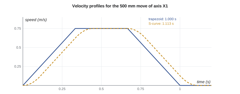
The workhorse of industrial motion is the trapezoidal velocity profile: accelerate at a constant rate to a cruise speed, cruise, then decelerate at a constant rate to stop. Its parameters are the distance D, the maximum speed and the maximum acceleration. The ramp time is \(t_a = v_{max}/a_{max}\), and the distance covered by both ramps together is \(a_{max} t_a^2\). If that is less than D, the profile cruises for \((D - a_{max}t_a^2)/v_{max}\); if not, the axis never reaches its maximum speed and the profile becomes a triangle, accelerating to a lower peak and immediately decelerating. For X1, with the limits from Lesson 2 of 0.75 m/s and 2.25 m/s², the 500 mm move is a trapezoid with equal thirds: a 0.333 s ramp, 0.333 s cruise and 0.333 s ramp, exactly 1.000 s. A short 80 mm move cannot reach full speed and becomes a triangle with a peak of 0.424 m/s and a total of 0.377 s, which is why short moves take proportionally longer.

Jerk and S-curves

A trapezoidal profile's acceleration jumps instantly from zero to its maximum and back. The rate of change of acceleration, called jerk, is infinite at those corners, and real mechanisms respond to such steps by ringing: the carriage, the fixture and the impeller on it are joined by finite stiffnesses, and a sudden change in force excites their natural frequencies. An S-curve profile limits jerk, ramping the acceleration up and down over a short time so that velocity changes smoothly. For X1 with a jerk limit of 20 m/s³, each acceleration ramp takes an extra 0.1125 s, and the move takes 1.113 s instead of 1.000 s. That costs 11 percent of the move time. Whether it is worth paying depends on the mechanism: for a stiff axis carrying a small load it is unnecessary, while for a tall, flexible gantry or a liquid-filled container it can save more time in settling than it costs in motion. On X1 the drill cannot start until the carriage has settled to within 0.05 mm, so Baywind tries both on the real axis and keeps whichever settles sooner.

Robots plan trajectories in the same way, with an extra choice: whether to interpolate in joint space or Cartesian space. A joint move, often programmed as a point-to-point or joint interpolated move, gives each joint a profile so that all joints start and finish together; the tool follows a curved path that is fast and avoids singularities but is hard to predict. A linear move makes the tool follow a straight line, solving inverse kinematics at every interpolation step; its path is predictable, which matters when inserting an impeller over an arbor, but it can pass near singularities as Lesson 9 described. Robot programmers use joint moves for travel through open space and linear moves for approaches and departures, with blending zones where one move rounds into the next without stopping.

Cascaded control

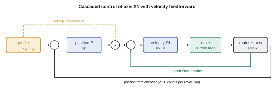
Servo drives control position with nested loops, as the figure shows. The innermost loop, inside the drive, controls motor current and therefore torque, typically at tens of kilohertz with a bandwidth of a kilohertz or more. Around it, a velocity loop compares the commanded speed with the speed measured from the encoder and sets the current command, usually with a proportional-integral (PI) controller. The outermost position loop compares the commanded position with the measured position and sets the velocity command, usually with proportional gain alone. Each loop is tuned to be several times slower than the one inside it, so that from the outer loop's point of view the inner loop is nearly ideal. This structure is easier to tune than a single PID controller acting on position, because each loop deals with a simpler problem, and it allows separate limits on current and speed.

The gain of the position loop, \(K_p\), has units of 1/s and a simple meaning: the velocity command per unit position error. With proportional control alone, an axis following a ramp at speed v must lag behind its command by \(v/K_p\) to generate that speed command. This lag is the following error. At 0.75 m/s with \(K_p = 20\) s⁻¹ it is 37.5 mm; tripling the gain to 60 s⁻¹ cuts it to 12.5 mm, but gains cannot be raised without limit because the mechanism's resonances and the encoder noise eventually make the loop unstable.

Feedforward

The cure for following error is not more feedback but feedforward. The profile generator knows the velocity it is asking for at every instant, so it can add that velocity directly to the velocity command, as the dashed path in the figure shows. The position loop then has to correct only the small errors the feedforward does not anticipate. Similarly, acceleration feedforward adds the torque needed to accelerate the known inertia directly to the current command. The program simulates X1 with a PI velocity loop and a P position loop, including a 9 A current limit. Without feedforward, the largest following error during the move is 37.4 mm at \(K_p = 20\) and 12.4 mm at 60, close to the simple \(v/K_p\) prediction. With velocity feedforward the error falls to 0.093 mm, more than a hundred times smaller, with the same feedback gains and therefore the same stability.

# Axis X1: a trapezoidal move profile, an S-curve alternative, and a cascaded position-velocity loop
import math

def trapezoid(D, vmax, amax):
    ta = vmax / amax
    if amax * ta * ta > D:                 # too short to reach vmax: triangular profile
        ta = math.sqrt(D / amax); vmax = amax * ta; tc = 0.0
    else:
        tc = (D - amax * ta * ta) / vmax
    return ta, tc, vmax, 2 * ta + tc
for D in (0.500, 0.080):
    ta, tc, v, T = trapezoid(D, 0.75, 2.25)
    shape = "triangle" if tc == 0 else "trapezoid"
    print(f"{1000*D:.0f} mm move: {shape}, ramp {ta:.3f} s, cruise {tc:.3f} s, peak {v:.3f} m/s, total {T:.3f} s")

# S-curve: jerk-limited ramps (jerk 20 m/s^3) for the same 500 mm move
J = 20.0; tj = 2.25 / J
ta_s = 0.75 / 2.25 + tj                        # each ramp lengthens by one jerk time
D_ramps = 0.75 * ta_s                          # distance covered in both ramps together (symmetric)
T_s = 2 * ta_s + (0.500 - D_ramps) / 0.75
print(f"S-curve with jerk {J:.0f} m/s^3: total {T_s:.3f} s (adds {T_s - 1.0:.3f} s, removes the step in acceleration)")

# Cascaded control: P position loop (Kp) outside a PI velocity loop (Kv, Ti), motor plus load inertia
Jt, kt = 4.31e-4, 0.80                         # total inertia (kg m^2), torque constant (N m/A)
lead = 0.020; ratio = 2 * math.pi / lead       # rad of motor per m of travel
Kp, Kv, Ti = 60.0, 0.35, 0.010                 # 1/s, A per rad/s, s
I_max = 9.0                                     # drive current limit (A)
def run(Kp, ff=True, dt=0.0001, T=1.4):
    x = v = integ = 0.0; worst = 0.0; t = 0.0; out = []
    while t < T:
        ta, tc, vm, Tt = trapezoid(0.5, 0.75, 2.25)
        if t < ta: xr, vr = 0.5 * 2.25 * t * t, 2.25 * t
        elif t < ta + tc: xr, vr = 0.5 * 2.25 * ta * ta + vm * (t - ta), vm
        elif t < Tt: tr = Tt - t; xr, vr = 0.5 - 0.5 * 2.25 * tr * tr, 2.25 * tr
        else: xr, vr = 0.5, 0.0
        w_cmd = ((vr if ff else 0.0) + Kp * (xr - x)) * ratio         # velocity feedforward plus position correction
        e = w_cmd - v * ratio
        integ += e * dt
        i = max(-I_max, min(I_max, Kv * (e + integ / Ti)))
        acc = kt * i / Jt / ratio                     # m/s^2 of the carriage
        v += acc * dt; x += v * dt
        worst = max(worst, abs(xr - x)); t += dt
    return worst, abs(0.5 - x)
for kp, ff in ((20.0, False), (60.0, False), (60.0, True)):
    fe, final = run(kp, ff)
    print(f"Kp {kp:4.0f} 1/s, velocity feedforward {'on ' if ff else 'off'}: largest following error {fe*1000:7.3f} mm, "
          f"error 0.4 s after the move {1e6*final:.1f} um")
counts = 2**20
print(f"Encoder {counts} counts per motor revolution = {1e6*lead/counts:.4f} um of travel per count")

500 mm move: trapezoid, ramp 0.333 s, cruise 0.333 s, peak 0.750 m/s, total 1.000 s
80 mm move: triangle, ramp 0.189 s, cruise 0.000 s, peak 0.424 m/s, total 0.377 s
S-curve with jerk 20 m/s^3: total 1.113 s (adds 0.113 s, removes the step in acceleration)
Kp   20 1/s, velocity feedforward off: largest following error  37.417 mm, error 0.4 s after the move 2.0 um
Kp   60 1/s, velocity feedforward off: largest following error  12.425 mm, error 0.4 s after the move 0.0 um
Kp   60 1/s, velocity feedforward on : largest following error   0.093 mm, error 0.4 s after the move 0.0 um
Encoder 1048576 counts per motor revolution = 0.0191 um of travel per count

Feedforward only works as well as the model behind it. If the inertia is estimated wrongly, acceleration feedforward adds the wrong torque, and the feedback must clean up the difference. That is one more reason the inertia calculation of Lesson 2 matters: Baywind's drive commissioning software will measure the inertia by moving the axis and fitting the response, and Owen will compare the measured value with his calculated 4.31 × 10⁻⁴ kg·m² as a check that the mechanism is assembled as designed. A large discrepancy usually means a binding guide, a misaligned coupling or a wrong screw lead in the drive's settings.

Encoders and resolution

Feedback is only as good as the measurement. X1's motor carries an absolute encoder with 2²⁰, or 1,048,576, counts per revolution; with a 20 mm screw lead, one count is 0.019 µm of carriage travel, far finer than the screw's own accuracy. Encoder resolution is rarely the limit on servo axes now. More often the limits are mechanical: the screw's lead error, its thermal growth as it warms up, backlash in couplings and the compliance between the motor and the load. Because the encoder sits on the motor, it measures the motor's position, not the carriage's. A linear scale on the carriage, used as a second feedback in a dual-loop arrangement, removes the screw from the measurement, at extra cost; X1's 0.05 mm settling requirement does not need one. Absolute encoders, which know their position at power-up, save the homing move that incremental encoders need after every power cycle.

Tuning in practice

Servo drives come with commissioning software that automates much of the tuning: it measures the frequency response of the axis, identifies resonances, and sets gains and notch filters to suppress them. The tuned result is then tested with the real profile and load, watching following error, current and settling on the drive's oscilloscope function. A good acceptance check for X1 is to run the 500 mm move a few hundred times with an impeller on the fixture and record the settling time to within 0.05 mm at the drill position; the requirement was set in the subsystem design and traces back to the cell's cycle time. If an axis that tuned well empty rings with an impeller on it, the inertia ratio of Lesson 2 is the first suspect.