
MEC-390 · Lesson 9 of 12 · 22 min
Feedback, steady-state error and disturbance rejection
Lesson 6 left Owen with a puzzle that Marco, the inspector, raises the moment he sees the simulation. With a proportional controller, the pressure loop settles 26 percent short of its setpoint. Marco signs test certificates that quote pressure to a hundredth of a bar, and a controller that cannot reach the pressure it is asked for is no use to him. The suction level loop has the opposite problem: it will reach its setpoint in quiet conditions, but every time the test flow changes, the level is pushed away and, with proportional control, stays away. This lesson explains both effects through the idea of system type and shows the three standard remedies: integral action, higher loop gain and feedforward.
Why use feedback at all
Feedback measures the output, compares it with what is wanted and acts on the difference. It costs a sensor, a controller and the risk of instability that Lesson 8 explored, so it must earn its place. It does so in three ways. It reduces the effect of disturbances, such as a change in test flow or a valve moving between test points. It reduces sensitivity to changes in the plant: a different pump on the stand, worn impellers or a different water temperature change the process gain, but a well-designed loop keeps the output where it should be anyway. And it can make an unstable or slow process stable and fast. An open-loop scheme, setting the drive speed from a table of pressure against speed, would work only as well as the table, and the table would be wrong the moment anything changed.
Error and the sensitivity function
Consider a loop with controller C(s), plant G(s), unity feedback for simplicity and a disturbance D(s) added at the plant output. The output is the sum of the responses to the setpoint and to the disturbance:
The function \(S(s) = 1/(1 + C(s)G(s))\) is the sensitivity function, and its complement \(T(s) = CG/(1 + CG)\) is the complementary sensitivity, the closed-loop transfer function. Since S + T = 1, they cannot both be small at the same frequency. Wherever the loop gain \(|CG|\) is large, S is small and the loop rejects disturbances and follows setpoints accurately; where the loop gain is small, disturbances pass through unopposed. Good control therefore means high loop gain at the frequencies where the disturbances and setpoint changes live, which for a test loop means low frequencies, down to steady state.
S also measures sensitivity to the plant in the sense its name suggests. If the plant gain changes by a small fraction \(\Delta G/G\), the closed-loop transfer function changes by \(S\,\Delta G/G\). A loop gain of 10 at steady state makes the closed loop ten times less sensitive to plant changes than the plant itself. Black's invention of the feedback amplifier in the 1920s rested on exactly this idea: with enough loop gain, the behaviour of a system depends on its feedback path, which can be made precise, rather than on its forward path, which cannot.
System type and the error constants
The steady-state error depends on how many integrators the loop transfer function contains, a number called the system type. Write \(L(s) = C(s)G(s)\) as \(K\,N(s)/(s^n\,D(s))\), with N(0) = D(0) = 1. Using the final value theorem on \(E(s) = R(s)/(1 + L(s))\) gives the steady error for standard inputs:
| Loop type n | Step input A/s | Ramp input A/s² | Parabola A/s³ |
|---|---|---|---|
| 0 | A/(1 + Kₚ), Kₚ = L(0) | ∞ | ∞ |
| 1 | 0 | A/Kᵥ, Kᵥ = lim sL(s) | ∞ |
| 2 | 0 | 0 | A/Kₐ, Kₐ = lim s²L(s) |
The pressure process has no integrator, so with a proportional controller the loop is type 0. Its position error constant is \(K_p = L(0) = 0.708K_c\), and a setpoint step leaves an error of \(1/(1 + 0.708K_c)\) of the step: 41 percent at \(K_c = 2\), 26 percent at 4 and 15 percent at 8. Raising the gain reduces the error but never removes it, and Lesson 8 showed that the gain cannot exceed 23.5 at all, where the error would still be 6 percent with a loop on the edge of instability. The valve position loop, by contrast, is type 1 because the actuator integrates; it reaches any constant setpoint exactly and follows a ramp with the constant error found in Lesson 7.
Disturbances and where they enter
Disturbances behave differently from setpoint changes, because what matters is the number of integrators between the controller and the point where the disturbance enters. The suction level loop shows this clearly. The tank integrates the difference between inflow and outflow, \(1/(As)\), so the plant itself is type 1, and with proportional control the level reaches its setpoint exactly after a setpoint change. But the disturbance, the outflow to the test pump, enters at the tank's input, before the integrator, on the same footing as the controller's own action. When the test flow rises from 90 to 120 m³/h, the fill valve must pass 30 m³/h more to keep the level steady. A proportional controller can only open the valve further if the error is held at a value that commands the extra opening.
With the fill valve passing 0.0004 m³/s per percent of output and the level transmitter giving 33.3 percent per metre, a gain \(K_c\) opens the valve by \(K_c \times 33.3 \times 0.0004\) m³/s for every metre of level error. Holding an extra 0.00833 m³/s therefore needs an error of
which is 156 mm at \(K_c = 4\) and 62 mm at \(K_c = 10\). Neither meets the ±50 mm specification. The general rule is that a loop rejects a constant disturbance completely only if there is an integrator between the error and the point where the disturbance enters, which means an integrator in the controller.
Integral action
A proportional-integral (PI) controller adds a term proportional to the integral of the error:
The integral term keeps changing the output for as long as any error remains, so the only possible steady state is zero error. In transfer function terms the controller adds a pole at the origin, raising the loop's type by one: the pressure loop becomes type 1 and reaches its setpoint exactly; the level loop's disturbance now passes an integrator in the controller and is rejected completely. The integral time \(T_i\) sets how fast the integral acts: in a time \(T_i\), a constant error makes the integral term grow by as much as the proportional term. The cost of integral action is phase lag, 90° at low frequencies, which erodes stability margins; Lessons 10 to 12 show how to choose \(T_i\) to keep the benefit and limit the cost.
# Steady-state error and disturbance rejection in the suction tank level loop LIC-101 (integrating process)
A = 4.0                 # tank area, m^2
kv = 0.0004             # fill valve LV-101: m^3/s per % of controller output
tv = 4.0                # valve and transfer pump lag, s
kl = 100/3.0            # level transmitter LT-101: % per m (0 to 3 m span)
def run(Kc, Ti=None, ff=False, T=1800.0, dt=0.05):
    h, qv, integ = 1.50, 0.025, 0.0          # level (m), valve flow (m^3/s), integral of error (%.s)
    bias = 0.025/kv                           # 62.5 % gives the normal 90 m^3/h
    worst, hist = 0.0, []
    for n in range(int(T/dt)):
        t = n*dt
        qout = 0.025 if t < 60 else 0.025 + 30/3600   # test flow steps from 90 to 120 m^3/h at t = 60 s
        e = (1.50 - h)*kl                    # level error, %
        if Ti: integ += e*dt
        u = (qout/kv if ff else bias) + Kc*(e + (integ/Ti if Ti else 0.0))
        u = min(max(u, 0.0), 100.0)
        qv += dt*(kv*u - qv)/tv; h += dt*(qv - qout)/A
        worst = min(worst, h - 1.50); hist.append(h)
    return worst, hist[-1] - 1.50
print("Disturbance: pump test flow steps from 90 to 120 m^3/h at t = 60 s")
print("  controller                       largest dip (mm)   offset after 30 min (mm)")
for label, Kc, Ti, ff in (("P, Kc = 4", 4.0, None, False), ("P, Kc = 10", 10.0, None, False),
                          ("PI, Kc = 4, Ti = 300 s", 4.0, 300.0, False), ("PI + feedforward from FT-201", 4.0, 300.0, True)):
    w, off = run(Kc, Ti, ff); off = 0.0 if abs(off) < 5e-5 else off
    print(f"  {label:30s}   {w*1000:8.0f}            {off*1000:8.1f}")
dq = 30/3600
print(f"\nP-only offset formula: e = dq/(Kc kl kv) = {dq/(4*kl*kv)*1000:.0f} mm at Kc = 4, {dq/(10*kl*kv)*1000:.0f} mm at Kc = 10")
# Setpoint offset of the pressure loop under P control (type 0 loop, plant gain 0.708)
for Kc in (2.0, 4.0, 8.0):
print(f"Pressure loop, Kc = {Kc:3.0f}: steady error {100/(1 + 0.708*Kc):.0f} % of a setpoint step")Disturbance: pump test flow steps from 90 to 120 m^3/h at t = 60 s controller largest dip (mm) offset after 30 min (mm) P, Kc = 4 -156 -156.2 P, Kc = 10 -62 -62.5 PI, Kc = 4, Ti = 300 s -117 0.0 PI + feedforward from FT-201 -7 0.0 P-only offset formula: e = dq/(Kc kl kv) = 156 mm at Kc = 4, 62 mm at Kc = 10 Pressure loop, Kc = 2: steady error 41 % of a setpoint step Pressure loop, Kc = 4: steady error 26 % of a setpoint step Pressure loop, Kc = 8: steady error 15 % of a setpoint step
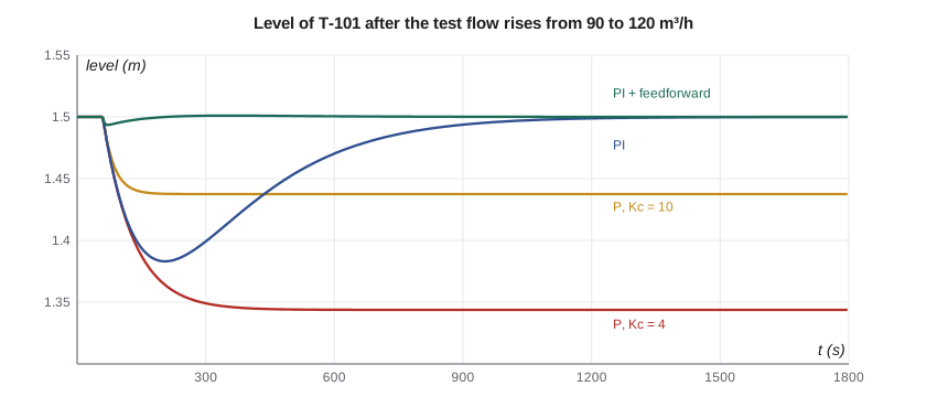
The simulation confirms the analysis. With P control the level settles 156 mm or 62 mm low. With PI control at \(K_c = 4\) and \(T_i = 300\) s, the level dips by 117 mm, then returns to within 5 mm of its setpoint about 15 minutes after the step. The dip still exceeds 50 mm, because integral action removes the offset but does not make the loop faster; the controller only learns about the disturbance after the level has already fallen.
Feedforward
When a disturbance can be measured, the controller need not wait for it to cause an error. TL-3's flow transmitter FT-201 measures the test flow, which is exactly the tank's outflow. Feedforward adds to the fill valve's command the opening that will pass that flow: \(u_{ff} = q_{out}/k_v\). If the feedforward were perfect, the inflow would always match the outflow and the level would never move; in practice the valve's 4 s lag and calibration errors leave a small residual, which the PI feedback trims away. The simulation shows a dip of only 7 mm with feedforward and PI together, an improvement of more than fifteen times.
Feedforward and feedback complement each other. Feedforward acts before an error appears but depends on a model and a measurement; it cannot correct for disturbances it does not see or for model errors. Feedback corrects everything that shows up in the measured output, including the imperfections of the feedforward, but only after it shows up. Because feedforward acts outside the loop, it does not change the loop's stability. Gilles likes the scheme for one more reason: if the flow transmitter fails, the controller can drop the feedforward term and carry on with PI alone.
Worked problem
Gain needed for a P-only level loop
What proportional gain would keep the P-only level offset within 50 mm for the 30 m³/h flow step, and why is that not a good solution?
Show solution
- Required \(K_c \ge 0.625/0.050 = 12.5\).
- The loop gain from level error to valve flow is then \(12.5 \times 33.3 \times 0.0004 = 0.167\) m³/s per metre.
Answer: At such a gain the fill valve would swing hard on every ripple of the level measurement, and any larger flow step would still exceed the limit. Integral action plus feedforward solves the problem at its root, at a modest gain.
Noise and the price of high gain
High loop gain rejects disturbances, but it also passes sensor noise straight to the actuator. The transfer function from measurement noise N(s) to the controller output is \(-C/(1 + CG)\), which at high frequencies, where the plant gain is small, approaches \(-C\). A proportional gain of 20 turns 0.5 percent of noise on the level signal into 10 percent of jitter on the fill valve, wearing its packing and actuator. This is why the specification for every loop is a balance: enough gain at low frequencies to reject disturbances, little enough at high frequencies to ignore noise and neglected dynamics. The shape of the loop gain across frequency, the subject of Lesson 11, is the tool for striking that balance.
Common mistakes
MistakeRaising proportional gain to remove steady-state error.
InsteadAdd integral action; finite gain in a type 0 loop always leaves an error.
MistakeAssuming an integrating plant rejects load disturbances.
InsteadRejection needs an integrator between the error and the point where the disturbance enters.
MistakeExpecting integral action to make a loop faster.
InsteadIt removes offset; feedforward or a faster loop reduces the initial deviation.
MistakeUsing feedforward alone.
InsteadCombine it with feedback to correct model errors and unmeasured disturbances.
MistakeForgetting that high gain amplifies measurement noise.
InsteadLimit high-frequency gain and filter only as much as stability allows.
Summary and key terms
- Feedback reduces the effect of disturbances and plant changes in proportion to the loop gain.
- The sensitivity S = 1/(1 + CG) and complementary sensitivity T = CG/(1 + CG) sum to one.
- System type, the number of integrators in the loop, sets the steady-state error to steps, ramps and parabolas.
- The P-controlled pressure loop is type 0 and leaves an error of 1/(1 + 0.708Kc); the level loop leaves 0.625/Kc m for a 30 m³/h flow step.
- PI control adds an integrator, removing steady error; the level dip falls from 156 mm to 117 mm and recovers.
- Feedforward from the flow transmitter cuts the level dip to 7 mm without affecting stability.
- Sensitivity function
- S = 1/(1 + L), the transfer function from output disturbance to output.
- Complementary sensitivity
- T = L/(1 + L), the closed-loop transfer function.
- System type
- The number of integrators in the loop transfer function.
- Position error constant
- Kp = L(0), which sets the steady error to a step in a type 0 loop.
- Load disturbance
- A disturbance entering at the plant input, such as a change in outflow.
- Offset
- A persistent steady-state error under proportional control.
- Integral action
- A controller term proportional to the integral of the error.
- Integral time
- The time in which integral action repeats the proportional action for a constant error.
- Feedforward
- Control action computed from a measured disturbance before it affects the output.
- Measurement noise
- Random error in a sensor signal that feedback passes to the actuator.
Practice problems
Work each problem on paper first, then reveal the answer to check.
A type 0 loop has L(0) = 9. What fraction of a setpoint step remains as error?
Show answer
1/(1 + 9) = 10 percent.
A type 1 loop has Kv = 5 s⁻¹. What is the steady error to a ramp of 2 units per second?
Show answer
2/5 = 0.4 units.
In the program, what P-only gain gives a 25 mm level offset?
Show answer
0.625/0.025 = 25.
With S = 0.1 at low frequency, how much does a 20 percent plant gain change alter the closed loop?
Show answer
About 2 percent.
Why does the integrating tank still need integral action in the controller?
Show answer
The outflow disturbance enters before the tank's integrator, so only a controller integrator rejects it.
What happens to the level loop if FT-201 fails and the feedforward is dropped?
Show answer
It reverts to PI: zero offset, but a dip of about 117 mm for the same flow step.
Lesson quiz · 5 questions
Score 60% or more to complete this lesson.
Create a free account to save your progress, take quizzes and earn a certificate.