Mechanical translational and rotational systems

The first parts of TL-3 that Owen models are mechanical: the stem of the throttling valve FV-301, which a hydraulic cylinder pushes against a return spring, and the drive train of motor, coupling and pump rotor, which the drive accelerates whenever the pressure controller asks for a new speed. Both are familiar from MEC-380, where he studied them as vibrating systems. The difference now is the question being asked. In vibration work the interest was in natural frequencies and resonance; for control the interest is in how the output responds to an input that the controller manipulates, and in which dynamics are fast enough to ignore.

The three translational elements

Every lumped mechanical model is built from three ideal elements. A mass m stores kinetic energy and obeys Newton's second law: the net force on it equals \(m\ddot x\). A spring of stiffness k stores potential energy and exerts a force proportional to the relative displacement of its ends, \(F = k(x_1 - x_2)\). A viscous damper with coefficient c dissipates energy and exerts a force proportional to the relative velocity, \(F = c(\dot x_1 - \dot x_2)\). Real components are approximations: a valve packing behaves partly as friction and partly as viscous drag, and a rubber mount is both spring and damper. The modeller chooses the idealization that captures the behaviour that matters at the time scale of interest.

Two conventions avoid most sign errors. First, choose a positive direction for each displacement and stick to it. Second, draw a free-body diagram of each mass showing every force acting on it, each drawn in the direction it acts when the displacement and velocity are positive. A spring stretched by a positive x pulls the mass back, so its force on the mass is −kx; a damper does the same with −cẋ. Summing forces and setting the total equal to mass times acceleration gives the equation of motion directly.

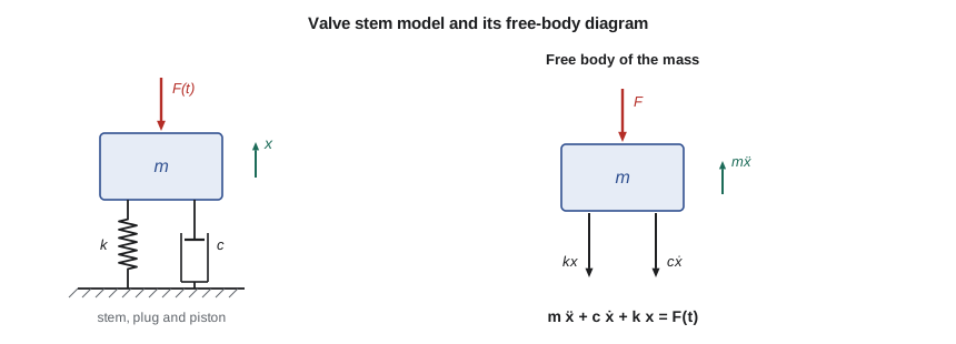
The valve stem model

The stem of FV-301, its plug and the actuator piston together have a mass of about 18 kg. A return spring with a stiffness of 60 kN/m closes the valve when hydraulic pressure is removed, which is the fail-safe direction Farah specified. Friction in the stem packing and viscous drag of oil in the cylinder are lumped into a damping coefficient of about 1,500 N·s/m. Taking x as the stem travel from the closed position and F as the net hydraulic force, the free-body diagram gives

Dividing by m and introducing the natural frequency and damping ratio from MEC-380 puts the equation in standard form:

For the stem, \(\omega_n = 57.7\) rad/s (9.19 Hz) and \(\zeta = 0.72\). A sudden 1,200 N increase in hydraulic force would eventually move the stem 1,200/60,000 = 20 mm, and with ζ = 0.72 it overshoots by less than 4 percent on the way. The whole response is over in about a tenth of a second. That is the first useful conclusion: the stem's mechanical dynamics are fast compared with everything else in the loop, so later lessons can often treat the stem as a pure spring, with travel proportional to force.

# Mechanical models on the TL-3 test loop: the valve actuator stem, the motor-pump drive train and a gear reducer
import math
# 1. Throttling valve FV-301: stem and plug mass, return spring and packing friction (treated as viscous)
m, k, c = 18.0, 60e3, 1500.0          # kg, N/m, N s/m
wn = math.sqrt(k / m); zeta = c / (2 * math.sqrt(k * m))
print(f"Valve stem: wn = {wn:.1f} rad/s ({wn/2/math.pi:.2f} Hz), zeta = {zeta:.2f}")
F = 1200.0                            # step in actuator force, N
print(f"Static travel for a {F:.0f} N step: {F/k*1000:.1f} mm")

def rk4(f, x, t, dt):
    k1 = f(t, x); k2 = f(t + dt/2, [a + dt/2*b for a, b in zip(x, k1)])
    k3 = f(t + dt/2, [a + dt/2*b for a, b in zip(x, k2)]); k4 = f(t + dt, [a + dt*b for a, b in zip(x, k3)])
    return [a + dt/6*(p + 2*q + 2*r + s) for a, p, q, r, s in zip(x, k1, k2, k3, k4)]

stem = lambda t, x: [x[1], (F - c*x[1] - k*x[0]) / m]   # state: position, velocity
x, dt, peak, tpk = [0.0, 0.0], 1e-4, 0.0, 0.0
for n in range(5000):
    x = rk4(stem, x, n*dt, dt)
    if x[0] > peak: peak, tpk = x[0], (n + 1)*dt
print(f"Simulated peak travel {peak*1000:.2f} mm at {tpk*1000:.0f} ms, overshoot {100*(peak*k/F - 1):.1f} %")

# 2. Motor, coupling with torque transducer, and pump rotor: two inertias joined by a torsional spring
Jm, Jp, kt = 0.090, 0.060, 6.0e3      # kg m^2 (pump value includes entrained water), N m/rad
w_t = math.sqrt(kt * (1/Jm + 1/Jp))
print(f"\nDrive train torsional mode: {w_t:.0f} rad/s = {w_t/2/math.pi:.1f} Hz")
print(f"Node position: {Jp/(Jm + Jp)*100:.0f} % of the shaft length from the motor end")
T = 59.7                              # rated torque at 1,760 rpm, N m
print(f"Twist of the coupling at rated torque: {T/kt*1000:.2f} mrad ({math.degrees(T/kt):.3f} deg)")
alpha = T / (Jm + Jp)
print(f"With rated torque and no load the rotor would accelerate at {alpha:.0f} rad/s^2,"
      f" reaching 1,760 rpm in {1760*2*math.pi/60/alpha:.2f} s")

# 3. Reflected inertia through the GR-5 reducer (18/76 teeth) driving the PC-150 sludge pump rotor
N = 76 / 18
J_motor, J_gear_in, J_load = 0.045, 0.004, 0.80   # kg m^2, motor side, input pinion, load side
J_eq = J_motor + J_gear_in + J_load / N**2
print(f"\nGear ratio {N:.3f}: load inertia {J_load} kg m^2 seen by the motor as {J_load/N**2:.4f} kg m^2")
print(f"Total inertia at the motor shaft {J_eq:.4f} kg m^2; the load is {J_load/N**2/J_eq*100:.0f} % of it")

Valve stem: wn = 57.7 rad/s (9.19 Hz), zeta = 0.72
Static travel for a 1200 N step: 20.0 mm
Simulated peak travel 20.76 mm at 79 ms, overshoot 3.8 %

Drive train torsional mode: 408 rad/s = 65.0 Hz
Node position: 40 % of the shaft length from the motor end
Twist of the coupling at rated torque: 9.95 mrad (0.570 deg)
With rated torque and no load the rotor would accelerate at 398 rad/s^2, reaching 1,760 rpm in 0.46 s

Gear ratio 4.222: load inertia 0.8 kg m^2 seen by the motor as 0.0449 kg m^2
Total inertia at the motor shaft 0.0939 kg m^2; the load is 48 % of it

Rotational elements

Rotating machinery uses the rotational counterparts of the same three elements. A rotor with polar moment of inertia J stores kinetic energy \(\tfrac12 J\omega^2\) and obeys \(\sum T = J\dot\omega\). A shaft or coupling of torsional stiffness \(k_t\) exerts a torque proportional to its twist, \(T = k_t(\theta_1 - \theta_2)\). A rotational damper, such as viscous drag in a bearing or the load of a pump, exerts a torque proportional to angular speed, \(T = b\omega\). The free-body diagram becomes a torque diagram, but the procedure is identical.

The inertia of a rotor is computed from its geometry or taken from the manufacturer's data. For a solid disc of mass m and radius r, \(J = \tfrac12 mr^2\); for a thin ring, \(J = mr^2\). Motor catalogues list rotor inertia directly. A pump impeller running full of water carries some of the water with it, and that entrained water adds to its effective inertia; for the TP-80 the impeller with its water is about 0.052 kg·m², the value Owen used in MEC-380, and with the shaft, sleeve and coupling half the pump side totals about 0.060 kg·m².

The motor, coupling and pump

The TL-3 drive train has the 11 kW motor (rotor inertia about 0.090 kg·m²) connected to the TP-80 through a flexible coupling with a torque transducer between the halves. Together, coupling and transducer have a torsional stiffness of about 6.0 kN·m/rad. A model with two inertias and a spring has two equations of motion, one for each rotor:

Here \(T_m\) is the motor torque, set by the drive, and \(b_p\omega_p\) is the pump's load torque linearized about the running speed (Lesson 4 derives \(b_p\)). Adding the two equations eliminates the coupling torque and gives the rigid-body motion of the whole train, \((J_m + J_p)\dot\omega = T_m - b_p\omega\). Subtracting them, each divided by its inertia, gives the relative motion: a torsional vibration in which the two rotors swing against each other at

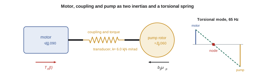
For TL-3 the torsional mode is at 408 rad/s, or 65 Hz, with a node 40 percent of the way from the motor to the pump. The program confirms Owen's hand calculation. This is far above any frequency the pressure controller will try to control: the pressure loop will need to act in a second or so, which corresponds to frequencies near 1 rad/s. For control purposes, then, the drive train is a single rigid inertia of 0.15 kg·m². Lucie adds a caution from her vibration work: the drive's own speed loop is much faster, and if its gains were set carelessly it could excite the torsional mode. That is a reason to keep the manufacturer's drive tuning rather than chase faster speed response.

The coupling twist at rated torque is small, about 10 mrad or 0.57°, but it is exactly what the torque transducer measures: the transducer is a calibrated torsion spring with strain gauges. A model that treated the coupling as rigid could not explain how the transducer works, which is a reminder that the right model depends on the question.

Gears and reflected inertia

Many machines drive their loads through gears or belts. An ideal gear pair with ratio \(N = \omega_{in}/\omega_{out}\) multiplies torque by N and divides speed by N, conserving power. When a load inertia \(J_L\) on the output shaft is accelerated, the torque needed at the input is \(J_L\dot\omega_{out}/N = J_L\dot\omega_{in}/N^2\). The load therefore looks, from the motor, like an inertia \(J_L/N^2\): it is reflected through the square of the ratio. Stiffness and damping on the output side reflect the same way.

Owen checks the GR-5 reducer that he designed in MEC-360, which drives the PC-150 progressive cavity sludge pump with an 18/76 tooth gear pair, a ratio of 4.222. The sludge pump's rotor and the output gear have about 0.80 kg·m², large because the rotor is long and heavy, but through the reducer it is seen by the motor as only 0.045 kg·m², slightly less than half the total inertia at the motor shaft. This is why reduction gears make heavy loads easy to start and why the choice of ratio also sets how quickly a drive can change speed.

Energy methods

For systems with one degree of freedom, writing the total energy is often quicker than drawing free-body diagrams. If damping and external forces are absent, kinetic plus potential energy is constant, and setting its time derivative to zero gives the equation of motion. For the stem, \(\tfrac12 m\dot x^2 + \tfrac12 kx^2 = \text{constant}\) differentiates to \(m\ddot x + kx = 0\). The method shines for systems with linkages, levers or rolling elements, where the kinematic relationships are easy to write in terms of energy but tedious to handle through forces. With damping and inputs present, the power balance generalizes the idea: the rate of change of stored energy equals the power supplied minus the power dissipated.

Energy thinking also explains the analogy between domains that Lesson 3 develops. In every domain, one pair of variables multiplies to give power: force and velocity, torque and angular speed, pressure and volume flow. Each domain has elements that store energy in two ways and an element that dissipates it, and once that is recognized, a hydraulic or thermal model can be written with the same confidence as a mechanical one.

Friction and other nonlinearities

Two nonlinear effects in the valve deserve mention because they cause real control problems. The first is static friction, or stiction, in the packing: the stem does not move until the force exceeds a breakaway value, then jumps. A valve with stiction makes a control loop hunt in a slow limit cycle that no tuning can remove; the fix is mechanical, by adjusting or replacing the packing, or by a valve positioner that pushes harder. The second is backlash in linkages, a dead zone in which the input moves without moving the output. Both are left out of the linear models of this course, but Owen notes them in his list of assumptions so that Gilles knows what to look for during commissioning.