
MEC-390 · Lesson 10 of 12 · 23 min
Root locus
Owen now knows that the pressure loop needs integral action and that its gain must stay well below the critical value of 23.5. What he does not yet have is a way to see how the closed-loop poles move as he changes the controller, so that he can place them where the time-response specifications of Lesson 7 want them. The root locus, introduced by Walter Evans in 1948, does exactly that. It is a plot of the closed-loop poles as one parameter, usually the gain, runs from zero to infinity. Computers draw it in an instant, but a few rules let an engineer sketch it by hand and, more importantly, understand why it has the shape it has and how adding a pole or zero reshapes it.
The angle and magnitude conditions
The closed-loop poles are the roots of \(1 + KL_0(s) = 0\), where \(L_0\) is the loop transfer function with the adjustable gain K taken out. Any point s on the locus must therefore satisfy \(KL_0(s) = -1\), which splits into two conditions:
The angle condition alone determines the shape of the locus: a point is on it if the angles from the open-loop zeros to the point, minus the angles from the open-loop poles, add to an odd multiple of 180°. The magnitude condition then tells which gain puts a closed-loop pole at that point. Geometrically, \(|L_0(s)|\) is the product of distances from the zeros divided by the product of distances from the poles, so K can be read off a sketch with a ruler.
Sketching rules
Six rules, all following from the angle condition, give the shape of the locus for positive K. The locus has as many branches as the loop has poles; each starts at an open-loop pole when K = 0 and, as K grows, either ends at an open-loop zero or goes to infinity. The branches are symmetric about the real axis. A point on the real axis is on the locus if the number of real poles and zeros to its right is odd. Branches going to infinity follow straight asymptotes at angles \((2k + 1)180^\circ/(n - m)\) from the real axis, where n is the number of poles and m the number of zeros, and the asymptotes meet at the centroid \(\sigma_a = (\sum p_i - \sum z_i)/(n - m)\). Two branches meeting on the real axis break away at a point where \(dK/ds = 0\). Branches cross the imaginary axis where the closed loop is marginally stable, at the frequency and gain the Routh test gives.
| Rule | Pressure loop with P control |
|---|---|
| Number of branches = number of poles | three, starting at −1.39, −2.0 and −10 |
| Real-axis segments: odd number of poles and zeros to the right | between −1.39 and −2.0, and to the left of −10 |
| Asymptote angles (2k + 1)180°/(n − m) | n − m = 3: 60°, 180°, 300° |
| Asymptote centroid | (−1.39 − 2.0 − 10)/3 = −4.46 |
| Break-away where dK/ds = 0 | s = −1.69, at K_c = 0.039 |
| Imaginary-axis crossing (Routh) | ±6.06j at K_c = 23.5 |
The locus of the pressure loop under proportional control
For proportional control the loop transfer function has the three poles of the plant and no zeros. The real axis between −1.39 and −2.0 is on the locus, since one pole lies to the right of every point there; so is the axis to the left of −10. The two slow poles move toward each other as the gain rises, meet at −1.69 when \(K_c\) is only 0.039, and break away into a complex pair. The third branch runs from −10 to the left along the axis. With three poles and no zeros, the complex branches follow asymptotes at ±60° from the centroid at −4.46, curving to cross the imaginary axis at ±6.06j when \(K_c = 23.5\), exactly the critical gain and frequency of Lesson 8.
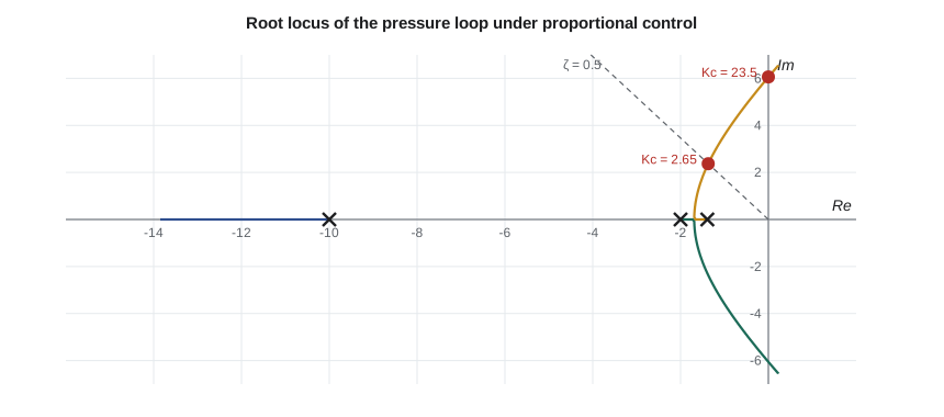
The locus shows at a glance why proportional control disappoints. To get well-damped poles, say ζ = 0.5 (16 percent overshoot), the gain must be kept at 2.65, where the dominant poles sit at \(-1.37 \pm 2.37j\). At that gain the loop settles in about 3 s, which is fine, but its steady error is 35 percent, which is not. Raising the gain to cut the error swings the poles toward the imaginary axis and the loop becomes oscillatory long before the error is acceptable. No point on this locus meets all the specifications at once. The controller must change the locus itself.
# Root locus of the discharge pressure loop: proportional control, then PI with the zero placed by the designer
import math, cmath
def pmul(a, b):
    r = [0.0]*(len(a) + len(b) - 1)
    for i, x in enumerate(a):
        for j, y in enumerate(b): r[i + j] += x*y
    return r
def roots(p):
    p = [c/p[0] for c in p]; n = len(p) - 1; z = [complex(0.4, 0.9)**k for k in range(n)]
    for _ in range(400):
        z = [zi - sum(c*zi**(n - k) for k, c in enumerate(p)) / math.prod(zi - zj for j, zj in enumerate(z) if j != i)
             for i, zi in enumerate(z)]
    return sorted(z, key=lambda w: w.real, reverse=True)
den = pmul(pmul([0.5, 1.0], [0.72, 1.0]), [0.1, 1.0]); Kp = 0.708
poles = [-2.0, -1/0.72, -10.0]
# Asymptotes and break-away point for P control (three poles, no zeros)
sigma = sum(poles)/3
print(f"Open-loop poles {', '.join(f'{p:.2f}' for p in poles)}; asymptotes at 60, 180, 300 deg from sigma = {sigma:.2f}")
# Break-away: d/ds of the denominator = 0 between the two slow poles
dpoly = [3*den[0], 2*den[1], den[2]]
bw = [r.real for r in roots(dpoly) if -2.0 < r.real < -1/0.72][0]
Kbw = -sum(c*bw**(3 - i) for i, c in enumerate(den))/Kp
print(f"Break-away from the real axis at s = {bw:.3f} with Kc = {Kbw:.3f}")
print("\n  Kc     closed-loop poles                              dominant zeta")
for Kc in (0.5, 2.0, 4.0, 8.0, 15.0, 23.5):
    cl = den[:]; cl[-1] += Kp*Kc; r = roots(cl); d = r[0]
    z = -d.real/abs(d)
    print(f"  {Kc:5.1f}  " + ",  ".join(f"{x.real:6.2f}{x.imag:+6.2f}j" for x in r) + f"     {z:.2f}")
# Gain for a dominant pair with zeta = 0.5 (bisection on Kc)
def zeta_of(Kc):
    cl = den[:]; cl[-1] += Kp*Kc; d = roots(cl)[0]; return -d.real/abs(d)
lo, hi = 2.0, 20.0
for _ in range(50):
    mid = (lo + hi)/2
    if zeta_of(mid) > 0.5: lo = mid
    else: hi = mid
print(f"\nKc = {lo:.2f} places the dominant poles at zeta = 0.50; the steady error is still {100/(1 + Kp*lo):.0f} %")

# PI control: C(s) = Kc (Ti s + 1)/(Ti s). The zero at -1/Ti is placed on the slowest plant pole (Ti = 0.72 s)
Ti = 0.72
num = [Kp*Ti, Kp]                          # Kp (Ti s + 1), multiplied by Kc below
denPI = pmul(den, [Ti, 0.0])
def zeta_PI(Kc):
    cl = denPI[:]; n = [Kc*c for c in num]; cl[-1] += n[-1]; cl[-2] += n[-2]
    r = roots(cl); r = [x for x in r if abs(x + 1/Ti) > 1e-3] or r
    d = r[0]; return -d.real/abs(d), r
lo, hi = 0.2, 15.0
for _ in range(50):
    mid = (lo + hi)/2
    if zeta_PI(mid)[0] > 0.5: lo = mid
    else: hi = mid
z, r = zeta_PI(lo)
print(f"PI with Ti = {Ti} s: Kc = {lo:.2f} gives zeta = 0.50, poles " + ", ".join(f"{x.real:.2f}{x.imag:+.2f}j" for x in r))
print(f" zero error to a setpoint step; dominant time constant about {-1/r[0].real:.2f} s")Open-loop poles -2.00, -1.39, -10.00; asymptotes at 60, 180, 300 deg from sigma = -4.46
Break-away from the real axis at s = -1.689 with Kc = 0.039
Kc closed-loop poles dominant zeta
0.5 -1.63 +1.03j, -1.63 -1.03j, -10.14 +0.00j 0.84
2.0 -1.44 +2.08j, -1.44 -2.08j, -10.51 +0.00j 0.57
4.0 -1.23 -2.87j, -1.23 +2.87j, -10.92 +0.00j 0.39
8.0 -0.89 -3.89j, -0.89 +3.89j, -11.60 +0.00j 0.22
15.0 -0.43 +5.06j, -0.43 -5.06j, -12.52 +0.00j 0.09
23.5 -0.00 -6.05j, -0.00 +6.05j, -13.38 +0.00j 0.00
Kc = 2.65 places the dominant poles at zeta = 0.50; the steady error is still 35 %
PI with Ti = 0.72 s: Kc = 1.46 gives zeta = 0.50, poles -0.83-1.44j, -0.83+1.44j, -10.33+0.00j
zero error to a setpoint step; dominant time constant about 1.20 sHow poles and zeros reshape the locus
Adding an open-loop pole pushes the locus to the right, toward instability: it adds an asymptote and swings the existing ones toward the imaginary axis. That is why each lag in a loop lowers its critical gain. Adding an open-loop zero pulls the locus to the left: a branch that would have gone to infinity ends at the zero instead, and the remaining asymptotes become more spread out. Controller design with the root locus is the art of placing controller poles and zeros so that the locus passes through the region of the s-plane where the specifications want the dominant poles.
PI control and zero placement
A PI controller, \(K_c(T_is + 1)/(T_is)\), adds a pole at the origin, which provides the integral action, and a zero at \(-1/T_i\), which the designer can place. The pole at the origin on its own would drag the locus to the right, making the loop slower and less stable. The zero is there to compensate. A widely used choice is to put the controller zero on top of the plant's slowest pole, here at −1.39, by choosing \(T_i = 0.72\) s. The zero and pole cancel in the loop transfer function, which becomes
The loop now has poles at 0, −2 and −10 and no zeros. Its locus has the same general shape as before, but its first branch starts from the origin, so the loop is type 1: the steady error to a setpoint step is zero at any gain. The program finds that \(K_c = 1.46\) places the dominant pair at ζ = 0.5, at \(-0.83 \pm 1.44j\), with the third pole at −10.3. The overshoot will be about 16 percent and the settling time about \(4/0.83 = 4.8\) s, inside the 10 s specification.
Cancellation is not perfect in practice, because the plant pole is only known approximately. If the true lag is 0.65 s or 0.80 s, a slow closed-loop pole remains close to the zero, producing a small, slowly decaying tail in the response. A small mismatch is harmless; the danger lies in trying to cancel a pole in the right half-plane, which can never be done reliably and leaves an unstable mode hidden inside the loop.
Worked problem
Effect of a faster integral
Gilles suggests a shorter integral time, \(T_i = 0.3\) s, to remove errors faster. Using the root locus rules, describe what happens to the locus and the achievable damping.
Show solution
- The controller zero moves to −3.33, to the left of both slow plant poles.
- The loop now has poles at 0, −1.39, −2 and −10 and a zero at −3.33: four poles, one zero, three asymptotes at 60°, 180° and 300°.
- The centroid is \((0 - 1.39 - 2 - 10 + 3.33)/3 = -3.35\), and the slow pole pair now includes the origin, so the dominant branches start nearer the axis.
Answer: The dominant poles stay closer to the imaginary axis, so for the same damping the gain must be lower and the loop is slower overall; integral action that is too strong makes a loop oscillatory. Running the same bisection as the program gives Kc = 0.34 for ζ = 0.5, with dominant poles at −0.48 ± 0.83j: settling takes about 8 s instead of 4.8 s.
Lead compensation
When integral action is not the issue but speed is, a lead compensator, \(C(s) = K_c(s + z)/(s + p)\) with the zero closer to the origin than the pole, pulls the locus to the left over a band of frequencies and lets the loop be both faster and well damped. Derivative action in a PID controller does something similar. For the valve position loop of Lesson 7, a lead zero placed near −40 rad/s, with its pole at −200, would allow a higher gain and faster positioning while keeping the overshoot below 5 percent, at the cost of more sensitivity to noise. Owen notes the option, but the 125 ms settling already meets the specification, so he leaves the position loop proportional.
Gain as the only parameter
The root locus is drawn for one parameter at a time, usually the gain, but any single parameter that enters the characteristic equation linearly can be used, such as the integral time or a plant constant. That makes the locus a tool for robustness as well as design: plotting the poles as the process gain varies over its expected range, for instance from a weak pump to a strong one, shows whether the loop stays acceptably damped at the extremes. Owen runs this check in Lesson 12, where the process gain varies across test points.
Common mistakes
MistakeIncluding real-axis segments with an even number of poles and zeros to the right.
InsteadOnly segments with an odd count belong to the locus.
MistakeForgetting that the locus is symmetric about the real axis.
InsteadComplex poles always come in conjugate pairs.
MistakeExpecting proportional control to meet damping and accuracy targets together.
InsteadAdd a controller zero and pole to reshape the locus.
MistakeCancelling an unstable plant pole with a controller zero.
InsteadCancellation is never exact; unstable modes must be stabilized, not cancelled.
MistakeChoosing a very short integral time to remove error quickly.
InsteadStrong integral action drags the locus toward instability.
Summary and key terms
- The root locus plots closed-loop poles as a gain varies; points on it satisfy ∠L₀ = 180° and K = 1/|L₀|.
- Branches start at open-loop poles and end at zeros or along asymptotes at (2k + 1)180°/(n − m) from the centroid.
- The pressure loop's P-control locus breaks away at −1.69 and crosses the imaginary axis at ±6.06j when Kc = 23.5.
- P control gives ζ = 0.5 at Kc = 2.65 but leaves a 35 percent steady error.
- PI with Ti = 0.72 s cancels the slowest plant pole; Kc = 1.46 gives ζ = 0.5 with zero steady error and about 4.8 s settling.
- Added poles push the locus right; added zeros pull it left; lead compensation trades noise sensitivity for speed.
- Root locus
- The paths of the closed-loop poles as one parameter varies from zero to infinity.
- Angle condition
- The requirement that ∠L₀(s) be an odd multiple of 180° at points on the locus.
- Magnitude condition
- The relation K = 1/|L₀(s)| giving the gain at a point on the locus.
- Asymptote
- A straight line that a branch approaches as the gain tends to infinity.
- Centroid
- The point on the real axis where the asymptotes meet.
- Break-away point
- Where two branches leave the real axis, at a local maximum of K.
- Pole-zero cancellation
- Placing a controller zero on a plant pole so that they cancel in the loop.
- Lead compensator
- A controller with a zero nearer the origin than its pole, adding phase lead.
- Dominant poles
- The closed-loop poles nearest the imaginary axis.
- Robustness
- The ability of a control system to perform acceptably when the plant changes.
Practice problems
Work each problem on paper first, then reveal the answer to check.
A loop has poles at 0, −1 and −4 and no zeros. Where is the asymptote centroid?
Show answer
(0 − 1 − 4)/3 = −1.67.
Which parts of the real axis are on the locus for poles at 0, −1 and −4?
Show answer
Between 0 and −1, and to the left of −4.
With two poles and one zero, how many asymptotes are there?
Show answer
One, along the negative real axis.
In the program, place the PI zero at −2 (Ti = 0.5 s) and keep the cancellation filter. What gain gives ζ = 0.5?
Show answer
Kc = 0.77, with dominant poles at −0.61 ± 1.06j: slower than cancelling the −1.39 pole, because the slowest lag remains in the loop.
L₀(s) = 0.6/((s − p₁)(s − p₂)(s − p₃)) and a point on the locus is 2, 3 and 5 units from the three poles. What gain puts a closed-loop pole there?
Show answer
|L₀| = 0.6/30 = 0.02, so K = 1/0.02 = 50.
Why does adding a lag to a loop lower its critical gain?
Show answer
The extra pole adds an asymptote and swings the branches toward the imaginary axis.
Lesson quiz · 5 questions
Score 60% or more to complete this lesson.
Create a free account to save your progress, take quizzes and earn a certificate.