
MEC-390 · Lesson 12 of 12 · 24 min
PID control in practice: the test loop capstone
The last weeks of Owen's term are spent turning the analysis into settings that Gilles can type into the TL-3 controller, and then watching the loop run. Most industrial control, on test stands as in refineries, paper mills and building systems, is done by PID controllers: proportional, integral and derivative action in one algorithm, available as a standard function block in every programmable controller. The theory of the earlier lessons tells Owen what each term does and where the limits lie. This lesson covers what the theory leaves out: the forms of the PID algorithm, the tuning rules engineers actually use, the nonlinear details that make or break a loop in service, and the capstone design of the TL-3 pressure and level loops.
The PID controller
The ideal, or standard, form of the PID controller is
The proportional term reacts to the present error, the integral term to its history, removing offset as Lesson 9 showed, and the derivative term to its trend, adding damping by anticipating where the error is heading. In the frequency domain, derivative action adds phase lead that can raise the phase margin and allow a faster loop. Its weakness is that it amplifies high-frequency noise without limit, so it is always implemented with a filter, typically \(T_ds/(1 + T_ds/N)\) with N between 5 and 20, which limits the high-frequency gain to \(NK_c\).
Controllers come in several forms, and settings from one form do not transfer directly to another. Besides the ideal form, many controllers use a parallel form with independent gains, \(K_p + K_i/s + K_ds\), and older or pneumatic-derived designs use a series form, \(K_c'(1 + 1/(T_i's))(1 + T_d's)\). Some express the gain as a proportional band, \(PB = 100/K_c\) percent, and the integral as repeats per minute, \(1/T_i\). Gilles checks the controller manual before entering any value; misreading the form is one of the commonest commissioning errors.
Practical refinements
Four refinements separate a textbook PID from one that works. First, derivative on measurement: applying the derivative to the measured value instead of the error avoids a huge spike, the derivative kick, every time the setpoint steps. Second, setpoint weighting: applying only a fraction b of a setpoint change to the proportional term reduces overshoot to setpoint changes without weakening the response to disturbances. Third, bumpless transfer: when an operator switches the loop from manual to automatic, the integral term is initialized so that the output does not jump. Fourth, and most important, anti-windup, which deserves its own discussion.
Integral windup
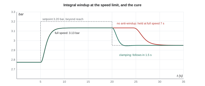
Every actuator has limits. The drive cannot exceed its maximum speed, a valve cannot open beyond fully open, and the fill valve's output is bounded between 0 and 100 percent. When the controller asks for more than the actuator can deliver, the error persists, and an unprotected integral term keeps growing, or winding up, long after the output has saturated. When the error finally reverses, the integral has to unwind before the output leaves its limit, and the process overshoots badly in the meantime.
TL-3 meets this situation regularly. During a run-out test the test engineer asks for a discharge pressure the pump cannot make at full speed. The program simulates a setpoint change from 2.77 to 3.20 bar; the pump at its maximum speed of 1,760 rpm can only reach 3.13 bar, so for 15 seconds the drive sits at its limit while the error stays at 0.07 bar. When the engineer lowers the setpoint to 2.95 bar, the unprotected controller holds the drive at full speed for another 7.3 s while its integral unwinds, and the pressure takes 7.8 s to settle. With anti-windup by clamping, which simply stops integrating while the output is saturated in the direction of the error, the pressure follows the new setpoint within 1.5 s. Other schemes, such as back-calculation, feed the difference between the requested and actual output back to the integrator; all of them prevent the integral from accumulating error the actuator cannot act on.
Discrete implementation
The TL-3 controller is a digital programmable controller that executes the PID algorithm every 50 ms. The integral becomes a running sum, \(I_k = I_{k-1} + (K_cT_s/T_i)e_k\), and the derivative a difference, filtered. Sampling adds delay, on average about half a sample period plus the computation time, so the sample time must be short compared with the loop's dynamics. A common rule is a sample time between a tenth and a twentieth of the closed-loop rise time, or below a tenth of the dominant time constant. At 50 ms against a pressure loop with time constants of 0.5 to 0.72 s and a crossover near 1 rad/s, the sampling costs less than 2° of phase and can be ignored in the design. The level loop could run a hundred times slower without harm.
Tuning rules
Engineers rarely derive controller settings from a full model. Instead they run a simple test on the process and apply a tuning rule. Three families are in wide use, and the program applies each to the pressure loop.
The Ziegler-Nichols ultimate-gain method, published in 1942, uses the critical gain and period found by raising a proportional gain until the loop oscillates steadily, or from the model as in Lesson 8: \(K_u = 23.5\), \(P_u = 1.04\) s. The rule sets a PI controller to \(K_c = 0.45K_u = 10.6\) and \(T_i = P_u/1.2 = 0.87\) s. The rules aim at a quarter-amplitude decay, which most modern practice considers too aggressive; Gilles also points out that driving a real test stand into sustained oscillation to find \(K_u\) is not something he will do with a customer's pump installed.
Reaction-curve methods fit a first-order-plus-dead-time (FOPDT) model, \(Ke^{-\theta s}/(\tau s + 1)\), to an open-loop step test. A convenient fit uses the times at which the response reaches 28.3 and 63.2 percent of its final change: \(\tau = 1.5(t_{63} - t_{28})\) and \(\theta = t_{63} - \tau\). For the pressure process the program finds K = 0.708, τ = 1.01 s and θ = 0.40 s: the three lags look, from outside, like one lag plus a delay. Cohen-Coon rules applied to this model give \(K_c = 3.36\) and \(T_i = 0.73\) s.
Lambda tuning, also called IMC tuning, lets the engineer choose the closed-loop time constant λ directly and computes the settings from the FOPDT model: \(K_c = \tau/(K(\lambda + \theta))\) and \(T_i = \tau\). It cancels the process lag with the controller zero, as Lesson 10 did with the root locus, and its single parameter λ trades speed against robustness in an understandable way. With λ = 1.0 s, comfortably longer than the dead time, the program gives \(K_c = 1.02\) and \(T_i = 1.01\) s.
# Capstone: tuning the TL-3 pressure loop PIC-201 and level loop LIC-101, with a discrete PI and anti-windup
import math
rho, g = 998.0, 9.81
def p_static(n):                       # steady discharge pressure (bar) at speed n (rpm), from the pump and system curves
    r = n/1760; q2 = max(40*r*r - 23.0, 0.0)/27200.0
    return rho*g*(23.0 + 14400*q2)/1e5
# 1. Ultimate-gain rules from Lesson 8 (Ku = 23.5, Pu = 1.04 s)
Ku, Pu = 23.5, 1.04
print(f"Ziegler-Nichols PI: Kc = {0.45*Ku:.1f}, Ti = {Pu/1.2:.2f} s   (aggressive: aims at quarter-amplitude decay)")
# 2. First order plus dead time fitted to the open-loop step (two-point method: 28.3 % and 63.2 % times)
taus, K = [0.5, 0.72, 0.1], 0.708
x = [0.0, 0.0, 0.0]; dt = 0.0005; t28 = t63 = None
for n in range(20000):
    x[0] += dt*(1 - x[0])/taus[0]; x[1] += dt*(x[0] - x[1])/taus[1]; x[2] += dt*(x[1] - x[2])/taus[2]
    if t28 is None and x[2] >= 0.283: t28 = n*dt
    if t63 is None and x[2] >= 0.632: t63 = n*dt; break
tau = 1.5*(t63 - t28); theta = t63 - tau
print(f"FOPDT fit: K = {K}, tau = {tau:.2f} s, dead time theta = {theta:.2f} s")
lam = 1.0
Kc_l, Ti_l = tau/(K*(lam + theta)), tau
print(f"Lambda tuning (lambda = {lam} s): Kc = {Kc_l:.2f}, Ti = {Ti_l:.2f} s")
cc_Kc = (1/K)*(tau/theta)*(0.9 + theta/(12*tau)); cc_Ti = theta*(30 + 3*theta/tau)/(9 + 20*theta/tau)
print(f"Cohen-Coon PI: Kc = {cc_Kc:.2f}, Ti = {cc_Ti:.2f} s")

# 3. Discrete PI (sample time 0.05 s) on the nonlinear loop, with the drive limited to 1,760 rpm
def run(Kc, Ti, antiwindup, T=40.0):
    Ts, h = 0.05, 0.0005
    n_act, p, pm = 1600.0, p_static(1600), p_static(1600)
    integ = 1600/18.0                  # integral term starts at the steady output for 1,600 rpm (%)
    u, out = integ, []
    for i in range(int(T/h)):
        t = i*h
        if i % int(Ts/h) == 0:         # controller executes every Ts
            sp = 3.20 if 5 <= t < 20 else (2.95 if t >= 20 else p_static(1600))
            e = (sp - pm)*100/6.0      # error in % of the 0-6 bar span
            v = Kc*e + integ
            u = min(max(v, 0.0), 1760/18.0)          # the drive cannot exceed 1,760 rpm
            if not (antiwindup and v != u):          # clamping: stop integrating while the output is saturated
                integ += Kc*Ts/Ti*e
            if antiwindup: integ = min(max(integ, 0.0), 1760/18.0)
        n_act += h*(18*u - n_act)/0.5; p += h*(p_static(n_act) - p)/0.72; pm += h*(p - pm)/0.1
        if i % 200 == 0: out.append((t, pm))
    hold = next(t for t, v in out if t >= 20 and v < 3.00) - 20
    under = 2.95 - min(v for t, v in out if t >= 20)
    return hold, max(under, 0.0), next((t for t, v in reversed(out) if abs(v - 2.95) > 0.03), 0) - 20
print("\nSetpoint 2.77 -> 3.20 bar at t = 5 s (not reachable at full speed), then 2.95 bar at t = 20 s")
print("  controller                    stays above 3.00 bar (s)   undershoot (bar)   settled within 0.03 bar (s)")
for lab, Kc, Ti, aw in (("lambda PI, no anti-windup", Kc_l, Ti_l, False), ("lambda PI, clamping", Kc_l, Ti_l, True),
                        ("Cohen-Coon PI, clamping", cc_Kc, cc_Ti, True), ("Z-N PI, clamping", 0.45*Ku, Pu/1.2, True)):
    hold, under, ts = run(Kc, Ti, aw)
    print(f"  {lab:28s}       {hold:5.1f}                  {under:5.3f}             {ts:5.1f}")

# 4. Level loop: lambda tuning for an integrating process, Kc = (2 lambda + theta)/(Ki (lambda + theta)^2), Ti = 2 lambda + theta
Ki, th = 0.0004*(100/3)/4.0, 4.0       # %/s per % of output, and the valve lag treated as dead time (s)
for lamL in (60.0, 120.0, 240.0):
    Kc = (2*lamL + th)/(Ki*(lamL + th)**2)
    print(f"Level loop, lambda = {lamL:4.0f} s: Kc = {Kc:5.2f}, Ti = {2*lamL + th:4.0f} s")

# 5. Robustness: margins of the lambda-tuned PI as the process gain changes between test points and pumps
import cmath
def margins(Kc, Ti, Kproc):
    pm = gm = None; prev = None
    for k in range(-6000, 4001):
        w = 10**(k/2000); s = 1j*w
        v = Kc*(1 + 1/(Ti*s))*Kproc/((0.5*s + 1)*(0.72*s + 1)*(0.1*s + 1))
        m, ph = abs(v), math.degrees(cmath.phase(v))
        if ph > 0: ph -= 360
        if prev and prev[0] >= 1 > m: pm = (w, 180 + ph)
        if prev and prev[1] > -180 >= ph: gm = (w, -20*math.log10(m))
        prev = (m, ph)
    return pm, gm
for Kproc, note in ((0.58, "1,450 rpm test point"), (0.708, "design point, 1,760 rpm"), (0.93, "larger impeller, +30 %")):
    (wc, pm), (wg, gm) = margins(Kc_l, Ti_l, Kproc)
print(f"Process gain {Kproc:5.3f} ({note}): crossover {wc:.2f} rad/s, PM {pm:.0f} deg, GM {gm:.1f} dB")Ziegler-Nichols PI: Kc = 10.6, Ti = 0.87 s (aggressive: aims at quarter-amplitude decay) FOPDT fit: K = 0.708, tau = 1.01 s, dead time theta = 0.40 s Lambda tuning (lambda = 1.0 s): Kc = 1.02, Ti = 1.01 s Cohen-Coon PI: Kc = 3.36, Ti = 0.73 s Setpoint 2.77 -> 3.20 bar at t = 5 s (not reachable at full speed), then 2.95 bar at t = 20 s controller stays above 3.00 bar (s) undershoot (bar) settled within 0.03 bar (s) lambda PI, no anti-windup 7.3 0.000 7.8 lambda PI, clamping 1.5 0.004 1.6 Cohen-Coon PI, clamping 0.7 0.118 3.0 Z-N PI, clamping 0.4 0.242 3.2 Level loop, lambda = 60 s: Kc = 9.08, Ti = 124 s Level loop, lambda = 120 s: Kc = 4.76, Ti = 244 s Level loop, lambda = 240 s: Kc = 2.44, Ti = 484 s Process gain 0.580 (1,450 rpm test point): crossover 0.60 rad/s, PM 78 deg, GM 25.2 dB Process gain 0.708 (design point, 1,760 rpm): crossover 0.74 rad/s, PM 74 deg, GM 23.5 dB Process gain 0.930 (larger impeller, +30 %): crossover 0.97 rad/s, PM 68 deg, GM 21.1 dB
| Method | Kc | Ti (s) | Behaviour in simulation |
|---|---|---|---|
| Ziegler-Nichols PI (ultimate gain) | 10.6 | 0.87 | fast; undershoots by 0.24 bar after a setpoint drop |
| Cohen-Coon PI (FOPDT) | 3.36 | 0.73 | undershoots by 0.12 bar after a setpoint drop |
| Root locus, ζ = 0.5 (Lesson 10) | 1.46 | 0.72 | PM 52°, 16 percent overshoot |
| Lambda, λ = 1.0 s | 1.02 | 1.01 | PM 74°, no overshoot, settles in about 2 s |
Choosing the pressure settings
The four methods span a factor of ten in gain, which is typical: tuning rules aim at different trade-offs, and none is right for every purpose. For TL-3 the priority is a pressure that settles smoothly to each new test point without overshoot, because overshoot means a test point that has to be re-stabilized. Speed beyond the 10 s settling requirement buys nothing. Owen recommends the lambda settings, \(K_c = 1.0\) and \(T_i = 1.0\) s. Their margins are generous: a phase margin of 74° and a gain margin of 23.5 dB at the design point.
The process gain is not constant. It falls to 0.58 at a 1,450 rpm test point, where the pressure is less sensitive to speed, and a TP-80 with the larger optional impeller would raise it by about 30 percent. The program recomputes the margins across that range: the phase margin stays between 68° and 78° and the gain margin above 21 dB. One set of settings serves every test point, so gain scheduling, changing the controller settings with the operating point, is not needed. Had the margins varied widely, the controller would have been given a table of settings indexed by speed.
The level loop
The level loop LIC-101 controls an integrating process: the tank integrates inflow minus outflow. The lambda rule for integrating processes, with process gain \(K_i = 0.00333\) percent per second per percent of output and the valve lag treated as a 4 s dead time, is \(K_c = (2\lambda + \theta)/(K_i(\lambda + \theta)^2)\) and \(T_i = 2\lambda + \theta\). Lambda is chosen from how much the level may move: the specification allows ±50 mm, and with the flow feedforward of Lesson 9 handling measured changes, the feedback only has to trim. Owen picks λ = 120 s, giving \(K_c = 4.76\) and \(T_i = 244\) s, close to the trial settings of Lesson 9. A longer λ would let the level drift more but move the fill valve more gently, which is often preferred for surge tanks; a shorter one tightens the level at the cost of a busier valve.
Cascade control
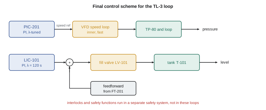
The pressure controller does not drive the motor directly; it sets the reference of the drive's own speed loop. That arrangement, one controller setting the setpoint of another, is cascade control. The inner loop is fast and corrects disturbances in its own part of the process, such as a supply voltage dip or a change in pump torque, before they reach the outer variable. The outer loop sees a well-behaved inner loop that it can treat as a simple lag. Cascade works when the inner loop is several times faster than the outer, which here it is by a wide margin. The valve position loop of Lesson 7 is used the same way when the flow controller sets the throttling valve's position.
Commissioning and safety
Gilles's commissioning plan follows a standard sequence. Check every transmitter's range and direction against the controller configuration, and confirm the action of each loop, so that rising pressure reduces speed and not the reverse. Run each loop in manual and make small output steps to confirm the model's gains and time constants. Enter the calculated settings, close the loop, and test setpoint steps and disturbance steps at several test points, recording the responses for the file. Test the limits: saturate each output deliberately and confirm that anti-windup works. Only then hand the loop to the test engineers.
Farah's specification makes one more point that Owen puts in bold in his report. Control loops are not safety systems. The high-pressure trip, the low suction-level pump stop and the emergency stop are implemented in a separate safety-rated system with its own sensors, designed and verified to machinery safety standards (in Canada, CSA Z432 for safeguarding together with ISO 13849-1 for safety-related control), and they act whatever the control loops are doing. A control loop that fails, saturates or is tuned badly must never be the only thing between the test stand and an unsafe condition.
At the end of the term the TL-3 loop runs its first full performance test on a TP-80. Each test point settles in under 10 s, the level stays within 12 mm through every flow change, and the test that used to take a morning is finished before the coffee break. Marco signs the certificate. Owen's report goes into the project file with the models, the settings and the commissioning records, so that the next engineer to retune the loop will know not just what the numbers are but why.
Common mistakes
MistakeEntering settings from one PID form into a controller that uses another.
InsteadCheck the controller's form and units: ideal, parallel or series; gain or proportional band; minutes or repeats.
MistakeUsing unfiltered derivative action on a noisy measurement.
InsteadFilter the derivative and apply it to the measurement, not the error.
MistakeLeaving out anti-windup because the actuator rarely saturates.
InsteadSaturation happens at start-up, at limits and during tests; always include anti-windup.
MistakeTreating tuning rules as exact.
InsteadThey are starting points with different aims; check margins and simulate.
MistakeRelying on a control loop for protection.
InsteadSafety functions belong in a separate, safety-rated system.
Summary and key terms
- PID control combines action on present error, accumulated error and error trend; derivative action needs a filter.
- Anti-windup stops the integral growing while the actuator is saturated; without it TL-3 stayed at full speed 7.3 s too long.
- Sample time should be short compared with loop dynamics; 50 ms costs under 2° in the pressure loop.
- An FOPDT fit of the pressure process gives K = 0.708, τ = 1.01 s, θ = 0.40 s.
- Lambda tuning (λ = 1 s) gives Kc = 1.02, Ti = 1.01 s, with PM 68° to 78° across the range of process gains.
- The level loop uses lambda tuning for an integrating process (Kc = 4.76, Ti = 244 s) with flow feedforward; safety functions stay separate.
- PID controller
- A controller acting on the error, its integral and its derivative.
- Derivative kick
- A spike in controller output caused by differentiating a setpoint step.
- Setpoint weighting
- Applying only part of a setpoint change to the proportional term.
- Bumpless transfer
- Switching between manual and automatic without a jump in output.
- Integral windup
- Growth of the integral term while the actuator is saturated.
- Anti-windup
- Any scheme that limits integral growth during saturation, such as clamping.
- FOPDT model
- A first-order-plus-dead-time approximation of a process for tuning.
- Lambda tuning
- A tuning method in which the designer chooses the closed-loop time constant λ.
- Cascade control
- An arrangement in which one controller sets the setpoint of another.
- Gain scheduling
- Changing controller settings according to the operating point.
Practice problems
Work each problem on paper first, then reveal the answer to check.
A controller shows a proportional band of 50 percent. What is its gain?
Show answer
Kc = 100/50 = 2.
An FOPDT process has K = 2, τ = 10 s and θ = 2 s. Find lambda PI settings for λ = 4 s.
Show answer
Kc = 10/(2 × 6) = 0.83; Ti = 10 s.
Using Ziegler-Nichols, find PI settings for Ku = 8 and Pu = 30 s.
Show answer
Kc = 3.6; Ti = 25 s.
In the program, set λ = 0.5 s for the pressure loop. What gain results?
Show answer
Kc = 1.01/(0.708 × 0.90) = 1.58.
For the level loop, what Kc and Ti does λ = 300 s give?
Show answer
Kc = 604/(0.00333 × 304²) = 1.96; Ti = 604 s.
Why must the pressure loop's action be checked during commissioning?
Show answer
If the action is reversed, the loop drives the error larger and runs to a limit.
Lesson quiz · 5 questions
Score 60% or more to complete this lesson.
Create a free account to save your progress, take quizzes and earn a certificate.