Harmonic forced vibration and resonance

Farah's question about the new baseplate is simple to ask and important to answer. The variable-speed TP-80 runs from 1,200 to 2,000 rpm, and the base's first mode, measured in Lesson 3, is at 33.1 Hz, or 1,988 rpm. What happens when the pump runs at that speed? And what happens at 1,760 rpm, the usual fixed speed, which is 11 percent below it? To answer, Owen needs the steady-state response of a damped system to a harmonic force. The result, the frequency response function, is the most important single idea in vibration engineering. It explains resonance, phase, the half-power bandwidth, and the reason that a small unbalance force can produce a large vibration.

The forced damped oscillator

A harmonic force \(F_0\cos\omega t\) acting on the damped single-degree-of-freedom system gives

The complete solution is the free vibration of Lesson 3, which decays, plus a steady-state part at the forcing frequency, which persists as long as the force acts. After a few time constants \(1/\zeta\omega_n\), only the steady state remains: \(x = X\cos(\omega t - \phi)\). Substituting gives the amplitude and phase lag:

The ratio \(X/(F_0/k)\) is the dynamic magnification factor: the amplitude divided by the deflection the same force would produce if applied slowly. It depends only on the frequency ratio r and the damping ratio ζ. In complex form, the response per unit force is the receptance \(H(\omega) = 1/(k - m\omega^2 + ic\omega)\), a complex number carrying both magnitude and phase. Measuring H over a range of frequencies is what a structural test engineer means by a frequency response function, or FRF.

Three regions of response

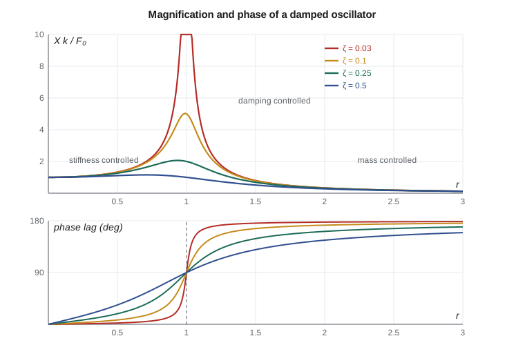
The curves fall into three regions. Well below resonance (r much less than 1) the response is stiffness controlled: X ≈ F₀/k, in phase with the force. Near resonance (r ≈ 1) it is damping controlled: the spring and inertia forces cancel, only damping resists the force, and \(X = F_0/(c\omega_n) = (F_0/k)/(2\zeta)\). The phase lag passes through 90° at resonance whatever the damping, which makes phase a reliable marker of resonance in measurements. Well above resonance (r much greater than 1) the response is mass controlled: \(X \approx F_0/(m\omega^2)\), and the mass moves opposite to the force, 180° out of phase. Lesson 5 exploits the mass-controlled region for isolation.

The peak of the magnification curve is at \(r = \sqrt{1 - 2\zeta^2}\), slightly below r = 1, with a height of \(1/(2\zeta\sqrt{1 - \zeta^2})\). For light damping this is close to \(Q = 1/(2\zeta)\), the quality factor. The baseplate's ζ of 0.0277 gives Q = 18.1: at resonance the base moves 18 times as far as it would under the same force applied statically.

Rotating unbalance as the force

The force from a rotating unbalance U = m_u e (the unbalance mass times its radius) is the centripetal force needed to carry it around: \(F_0 = U\omega^2\). Unlike a fixed force, it grows with the square of speed. For a system excited by its own unbalance, the response can be written as

which tends to 1 at high speed: well above resonance, the machine's mass m moves just enough to keep the combined centre of mass fixed. Lesson 11 meets this again in the Jeffcott rotor. Lesson 6 shows that the G6.3 balance grade allows the TP-80 impeller a residual unbalance of 325 g·mm, which produces 11.0 N at 1,760 rpm. That is the force used in the program.

# Forced response of the TP-80 baseplate mode (Lesson 3) to the impeller's rotating unbalance
import math, cmath
fn, zeta, m = 33.13, 0.0277, 113.0          # baseplate mode from the bump test
k = m * (2 * math.pi * fn)**2
U = 325e-6                                  # residual unbalance, kg m (325 g mm, Lesson 6)
def response(rpm):
    w = 2 * math.pi * rpm / 60
    F0 = U * w**2                           # unbalance force amplitude, N
    r = w / (2 * math.pi * fn)
    H = 1 / (k * complex(1 - r**2, 2 * zeta * r))   # receptance, m/N
    X = F0 * H
    return r, F0, abs(X), -math.degrees(cmath.phase(X)), abs(X) * w
print(f"Mode: k = {k/1e6:.2f} MN/m, Q = 1/(2 zeta) = {1/(2*zeta):.1f}")
print(" rpm    r     force N   amp um   lag deg   vel mm/s RMS")
for rpm in (1200, 1500, 1760, 1900, 1988, 2000, 2100, 2400):
    r, F0, X, ph, V = response(rpm)
    print(f"{rpm:5d} {r:5.3f} {F0:9.1f} {X*1e6:8.1f} {ph:8.1f} {V/math.sqrt(2)*1e3:9.2f}")
r, F0, X, ph, V = response(1760)
print(f"\nAt 1,760 rpm the dynamic magnification is {X*k/F0:.2f}")
# Half-power bandwidth check on a measured sweep: frequencies where the amplitude is peak/sqrt(2)
f1, f2 = 32.22, 34.06
print(f"Half-power points {f1} and {f2} Hz -> zeta = {(f2-f1)/(2*fn):.4f}")
# Options for a variable-speed customer who wants 1,200 to 2,000 rpm
for name, fnew, znew in (("as built", fn, zeta), ("grouted base, 45 Hz", 45.0, 0.04), ("added stiffener, 40 Hz", 40.0, 0.03)):
    kk = m * (2 * math.pi * fnew)**2
    worst = 0
    for rpm in range(1200, 2001, 10):
        w = 2 * math.pi * rpm / 60; rr = w / (2 * math.pi * fnew)
        X = U * w**2 / (kk * abs(complex(1 - rr**2, 2 * znew * rr)))
        worst = max(worst, X * w / math.sqrt(2) * 1e3)
    margin = (fnew * 60 - 2000) / 2000 * 100
    print(f"{name:24s}: worst velocity in the speed range {worst:5.2f} mm/s RMS, margin above 2,000 rpm {margin:5.1f} %")

Mode: k = 4.90 MN/m, Q = 1/(2 zeta) = 18.1
 rpm    r     force N   amp um   lag deg   vel mm/s RMS
 1200 0.604       5.1      1.6      3.0      0.15
 1500 0.755       8.0      3.8      5.5      0.42
 1760 0.885      11.0     10.2     12.8      1.33
 1900 0.956      12.9     25.9     31.5      3.65
 1988 1.000      14.1     51.9     90.2      7.64
 2000 1.006      14.3     51.0    102.5      7.55
 2100 1.056      15.7     24.7    153.2      3.84
 2400 1.207      20.5      9.1    171.7      1.61

At 1,760 rpm the dynamic magnification is 4.51
Half-power points 32.22 and 34.06 Hz -> zeta = 0.0278
as built                : worst velocity in the speed range  7.65 mm/s RMS, margin above 2,000 rpm  -0.6 %
grouted base, 45 Hz     : worst velocity in the speed range  0.51 mm/s RMS, margin above 2,000 rpm  35.0 %
added stiffener, 40 Hz  : worst velocity in the speed range  0.96 mm/s RMS, margin above 2,000 rpm  20.0 %

The table answers Farah's question. At 1,760 rpm, r = 0.885 and the magnification is 4.5: the 11 N force produces 10 µm and 1.33 mm/s RMS. That is acceptable but already amplified. As speed rises toward 1,988 rpm, the amplitude climbs to 52 µm and the velocity to 7.6 mm/s RMS, enough to damage bearings and seals. The phase lag passes through 90° at that speed. Above resonance, at 2,400 rpm, the response falls back to 1.6 mm/s with the phase near 180°. A pump that only passes through resonance during a start may be acceptable, but one that a control system might hold at 1,990 rpm for hours is not.

The half-power bandwidth

A forced test gives a second way to measure damping. On the magnification curve, the half-power points are the frequencies at which the amplitude is \(1/\sqrt2\) of the peak (the power, proportional to amplitude squared, is half). For light damping they are spaced by

Owen ran a slow sweep with the variable-speed motor on the test stand, recording the vibration at each speed, and found half-power points at 32.22 and 34.06 Hz. The program gives ζ = 0.0278, matching the bump test of Lesson 3 within a fraction of a percent. Two independent methods agreeing so well gives Lucie confidence in the model. In practice, run-up and coast-down recordings on large machines are used in exactly this way to locate critical speeds and estimate their damping (Lesson 11).

Design options for the variable-speed base

The last part of the program compares three versions of the baseplate over the full 1,200 to 2,000 rpm range. As built, the worst case is 7.65 mm/s RMS at resonance, and the mode sits just inside the top of the speed range. Adding a stiffener between the pump feet raises the mode to about 40 Hz, 20 percent above the top speed, and the worst velocity in the range falls to 0.96 mm/s. Grouting the base on a concrete foundation, as the installation manual recommends, raises the mode to about 45 Hz and the worst case to 0.51 mm/s. The cheapest option for the customer is grouting; the most robust option for Tidewater, which cannot control how bases are installed, is the stiffener. Farah adds it to the drawing.

Two other options were discussed and rejected. Lowering the mode below 1,200 rpm (20 Hz) would need a very flexible base, and the pump would pass through resonance at every start. Restricting the drive so that it skips the band from 1,900 to 2,080 rpm is possible, since most drives have programmable skip frequencies, but it relies on the customer's settings and does not protect a fixed-speed pump if a future impeller change raises its speed. Skip bands are a useful field fix and a poor design choice.

Response to other harmonic inputs

Not every harmonic force acts on the mass. A pump can be excited through its foundation (base excitation, Lesson 5), through pressure pulsations in its piping, or by a force that does not grow with speed, such as an electromagnetic force at twice line frequency. In each case the same magnification curve applies, multiplied by the appropriate force law. Pressure pulsations at vane-pass frequency, for instance, have roughly constant amplitude for a given flow, so a pipe mode near 176 Hz would show a magnification curve with no ω² factor. Owen's notebook now contains a short table: identify the force, its frequency and how its amplitude varies with speed, then apply the magnification for the mode in question.

A periodic but non-sinusoidal force, such as the pulse of a reciprocating pump, can be expanded as a Fourier series of harmonics. Because the system is linear, the response is the sum of the responses to each harmonic, each with its own magnification. A mode near the third harmonic of plunger frequency can respond strongly even if the fundamental is far away. Lesson 12 applies the same principle in reverse: the spectrum of a measured vibration separates a complicated motion into harmonic components whose sources can be identified.