
MEC-380 · Lesson 1 of 12 · 24 min
Vibration fundamentals and models
Owen Clarke's fourth work term at Tidewater Pump Works in Moncton begins in a different part of the plant. In MEC-360 he sat with Farah Siddiqui in the design group, sizing the TP-80 shaft, its bearings and the cover bolts. This term he has joined the test and reliability group, run by Lucie Arsenault, the company's vibration specialist. Every pump that leaves the plant runs on the test stand first, and every one of them is checked for vibration before it is crated. Lucie's first instruction is blunt: a pump that meets its head and flow but shakes is not a good pump. Vibration wears bearings and seals, loosens bolts, cracks welds and piping, carries noise into buildings and, at worst, destroys the machine. Over the next twelve lessons Owen will learn to predict vibration on paper, measure it on the stand and in the field, and fix it when customers call.
What vibration is
Vibration is the oscillation of a mechanical system about an equilibrium position. Three ingredients are always present: something that stores kinetic energy (mass or rotary inertia), something that stores potential energy (a spring, an elastic shaft, gravity acting on a pendulum or a column of water), and something that dissipates energy (damping, from friction, material hysteresis, fluid drag or deliberate dampers). When the system is displaced and released, energy passes back and forth between the kinetic and potential stores while damping removes a little on each cycle. When an outside force acts repeatedly, such as the rotating unbalance of an impeller, the system is driven at the frequency of that force and can respond strongly if that frequency is close to one of its own natural frequencies.
Engineers group vibration problems in a few ways. Free vibration happens after an initial disturbance with no continuing force: the ring of a baseplate after a hammer tap. Forced vibration is driven by a continuing input: the 1,760 rpm unbalance force of a pump. Vibration is undamped or damped, linear or nonlinear, and deterministic or random. Most machinery problems can be treated as linear, lightly damped and deterministic, which is why the simple models in this course work so well. Random vibration, such as the broad-band hiss of cavitation or turbulence, is introduced in Lesson 12 through measurement rather than theory.
Degrees of freedom
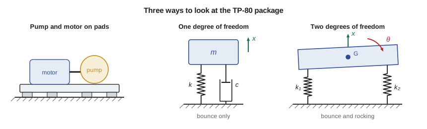
The number of degrees of freedom of a system is the number of independent coordinates needed to describe its position at any instant. A mass on a spring that can only move up and down has one. The TP-80 package on its baseplate can translate in three directions and rotate about three axes, so as a rigid body on mounts it has six. A flexible shaft or a pipe span has, strictly, an infinite number, because every point along it can deflect independently. Modelling means choosing how many degrees of freedom to keep. Lucie's rule is to keep the fewest that capture the behaviour you care about: a single degree of freedom model often predicts the one resonance that matters, a two- or three-degree model handles coupled motions, and continuous models of beams and shafts (Lesson 10) handle structures whose mass and stiffness are spread out.
A lumped model places all mass at points and represents all stiffness by massless springs. Real parts have both mass and flexibility everywhere, so the lumping always involves judgement. A short, stiff pump shaft carrying a heavy impeller is well represented by a massless spring and a point mass; a long, slender pipe span is not, and must be treated as a continuous beam or split into many lumps. The test of a good model is that its predictions agree with measurements, and the test stand gives Owen plenty of measurements to compare with.
Harmonic motion
The simplest vibration is harmonic, a motion that varies as a sine or cosine in time. If the displacement of the bearing housing is
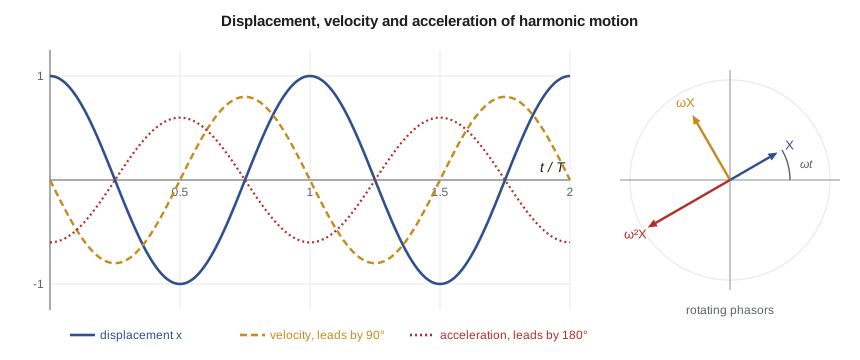
then X is the amplitude, ω the circular frequency in radians per second, and φ the phase angle. The frequency in hertz is \(f = \omega/2\pi\) and the period is \(T = 1/f\). A pump turning at 1,760 rpm has a running-speed frequency of 29.33 Hz and a period of 34.1 ms. Differentiating gives the velocity and acceleration:
The velocity amplitude is ωX and the acceleration amplitude ω²X. Velocity leads displacement by 90° and acceleration leads it by 180°. These relations are the most used formulas in vibration work, because sensors measure one quantity and standards often specify another. An accelerometer measures acceleration; a velocity pickup, velocity; a proximity probe, the displacement of a shaft relative to its bearing. Converting between them requires the frequency, and the conversion is only exact for a single harmonic.
Harmonic motion is conveniently represented as the projection of a rotating vector, or phasor, of length X rotating at ω. In complex notation \(x = \operatorname{Re}(\bar X e^{i\omega t})\), where the complex amplitude \(\bar X = X e^{-i\phi}\) carries both magnitude and phase. Differentiation becomes multiplication by iω, which is why velocity is 90° ahead of displacement. Two vibrations at the same frequency add as phasors, not as amplitudes: Lesson 6 relies on this to balance rotors.
Peak, peak-to-peak and RMS
An amplitude can be stated as the peak value, the peak-to-peak value (twice the peak for a sine) or the root-mean-square (RMS) value, which for a sine is the peak divided by √2. RMS is related to energy and is the basis of most international machinery standards, including the ISO 20816 series used in Lesson 12. Proximity-probe displacement is usually quoted peak-to-peak, because the probe sees the full swing of the shaft. Mixing these conventions is a common source of disputes between customers and suppliers, so Tidewater's test reports state the convention beside every number.
Canadian plants mostly follow ISO practice and quote velocity in millimetres per second RMS. Some customers, especially those who buy American-built equipment or follow American insurance guidance, quote velocity in inches per second peak and displacement in mils (thousandths of an inch) peak-to-peak, so Lucie's reports give both.
# Harmonic motion at the TP-80 bearing housing, unit conversions and equivalent springs
import math
f = 1760 / 60                      # running speed, Hz
w = 2 * math.pi * f                # rad/s
v_rms = 2.8e-3                     # measured velocity, m/s RMS (2.8 mm/s)
v_pk = v_rms * math.sqrt(2)
x_pk = v_pk / w                    # displacement amplitude, m
a_pk = v_pk * w                    # acceleration amplitude, m/s^2
print(f"Running speed {f:.2f} Hz, omega = {w:.1f} rad/s, period {1000/f:.1f} ms")
print(f"Velocity  {v_rms*1e3:.2f} mm/s RMS = {v_pk*1e3:.2f} mm/s peak = {v_pk/0.0254:.3f} in/s peak")
print(f"Displacement {x_pk*1e6:.1f} um peak = {2*x_pk*1e6:.1f} um pk-pk = {2*x_pk/25.4e-6:.2f} mils pk-pk")
print(f"Acceleration {a_pk:.3f} m/s^2 peak = {a_pk/9.81:.3f} g peak")
# Same velocity at vane-pass frequency (6 vanes) gives a very different displacement and acceleration
fv = 6 * f; wv = 2 * math.pi * fv
print(f"At vane pass {fv:.0f} Hz the same 2.8 mm/s is {v_pk/wv*1e6:.1f} um peak and {v_pk*wv/9.81:.2f} g peak")

# Adding two vibrations at the same frequency: phasors add as complex numbers
z1 = 2.0 * complex(math.cos(0), math.sin(0))
z2 = 1.5 * complex(math.cos(math.radians(120)), math.sin(math.radians(120)))
z = z1 + z2
print(f"2.0 mm/s at 0 deg + 1.5 mm/s at 120 deg = {abs(z):.2f} mm/s at {math.degrees(math.atan2(z.imag, z.real)):.0f} deg")

# Equivalent stiffness of the package mounting
k_pad = 2.2e6                      # each rubber pad, N/m
k_parallel = 4 * k_pad             # four pads share the load
k_frame = 12e6                     # flexibility of the floor frame under them, N/m
k_series = 1 / (1 / k_parallel + 1 / k_frame)
print(f"\nFour pads in parallel: {k_parallel/1e6:.1f} MN/m; in series with the frame: {k_series/1e6:.2f} MN/m")
# Level in decibels relative to 1 nm/s (ISO 1683 velocity reference)
print(f"Velocity level: {20*math.log10(v_rms/1e-9):.1f} dB re 1 nm/s")Running speed 29.33 Hz, omega = 184.3 rad/s, period 34.1 ms Velocity 2.80 mm/s RMS = 3.96 mm/s peak = 0.156 in/s peak Displacement 21.5 um peak = 43.0 um pk-pk = 1.69 mils pk-pk Acceleration 0.730 m/s^2 peak = 0.074 g peak At vane pass 176 Hz the same 2.8 mm/s is 3.6 um peak and 0.45 g peak 2.0 mm/s at 0 deg + 1.5 mm/s at 120 deg = 1.80 mm/s at 46 deg Four pads in parallel: 8.8 MN/m; in series with the frame: 5.08 MN/m Velocity level: 128.9 dB re 1 nm/s
The first reading Owen takes on the stand is 2.8 mm/s RMS on the outboard bearing housing at running speed. The program shows that this is 3.96 mm/s peak, or 0.156 in/s peak, and corresponds to a displacement of only 21.5 µm peak (43 µm or 1.69 mils peak-to-peak) and an acceleration of 0.73 m/s², about 0.074 g. The same velocity at the 176 Hz vane-pass frequency would be only 3.6 µm of displacement but 0.45 g of acceleration. This is why velocity is the preferred quantity for judging machinery: across the range of about 10 Hz to 1 kHz, a given velocity represents roughly the same severity of stress and wear, while displacement exaggerates low-frequency vibration and acceleration exaggerates high-frequency vibration.
Worked problem
Adding two vibrations at the same frequency
The impeller's residual unbalance produces 2.0 mm/s at the bearing at a phase of 0°, and a slight misfit of the coupling produces 1.5 mm/s at running speed with a phase of 120°. What does the sensor read?
Show solution
- Write each as a phasor: \(2.0\angle 0^\circ = 2.0 + 0i\) and \(1.5\angle 120^\circ = -0.75 + 1.30i\).
- Add: \(1.25 + 1.30i\).
- Magnitude \(\sqrt{1.25^2 + 1.30^2} = 1.80\) mm/s, phase \(\arctan(1.30/1.25) = 46^\circ\).
Answer: The sensor reads 1.80 mm/s at 46°, less than either source added arithmetically (3.5 mm/s) would suggest. Vibrations at the same frequency can partly cancel; at different frequencies their RMS values combine as the square root of the sum of squares.
Springs and their combinations
A linear spring produces a force proportional to its deflection, \(F = kx\), and stores energy \(\tfrac12 kx^2\). Many machine elements behave as springs. Some common stiffness formulas follow:
| Element | Stiffness | Notes |
|---|---|---|
| Axial bar, length L, area A | EA/L | pump hold-down bolt in tension |
| Torsional shaft, length L | GJ/L, with J = πd⁴/32 | shaft between coupling and impeller |
| Cantilever, tip load | 3EI/L³ | gauge on a pipe nipple |
| Simply supported beam, central load | 48EI/L³ | baseplate member between supports |
| Fixed-fixed beam, central load | 192EI/L³ | stiffened frame member |
| Coil spring | Gd⁴/(8D³N_a) | isolator spring (MEC-360, Lesson 12) |
Springs that share a load and deflect together act in parallel, and their stiffnesses add: four identical rubber pads under a baseplate give four times the stiffness of one. Springs that carry the same force one after the other act in series, and their flexibilities (the reciprocals of stiffness) add. The softer spring in a series pair dominates, so a stiff isolator sitting on a flexible floor beam behaves like the beam. The program shows this for the TP-80 package: four pads of 2.2 MN/m in parallel give 8.8 MN/m, but resting on a floor frame with a stiffness of 12 MN/m, the combination is only 5.08 MN/m. Owen will meet this again and again: the support structure is part of the vibrating system.
Masses also need care. A mass that moves with velocity v stores kinetic energy \(\tfrac12 mv^2\); a rotor with polar inertia J turning at angular speed θ̇ stores \(\tfrac12 J\dot\theta^2\). When parts move at different speeds, as in a gear train or a lever, an equivalent mass at a chosen coordinate is found by equating kinetic energies. A mass moving at twice the speed of the reference coordinate counts four times. The same idea gives the effective mass of a spring or beam in Lesson 2.
Damping
Damping removes energy and limits the response at resonance. Viscous damping, a force proportional to velocity \(F = c\dot x\), is the mathematical workhorse because it keeps the equations linear. Real mechanisms include dry (Coulomb) friction at joints, hysteresis in rubber and in steel, fluid films in journal bearings, and air or water drag. In machinery structures the damping is usually small, often 1 to 5 percent of the critical value defined in Lesson 3, and it is very hard to calculate. That is why Lucie measures damping rather than predicting it, and why the bump test of Lesson 3 is one of the first things done on any new baseplate design.
Sources of vibration in pumps
Before any model, Lucie asks what forces act on the machine and at what frequencies. In a centrifugal pump the main sources are: residual unbalance of the impeller, coupling and motor rotor, at running speed (1×); misalignment between motor and pump shafts, mainly at 1× and 2×; hydraulic pulsations as impeller vanes pass the volute tongue or diffuser vanes, at vane-pass frequency (number of vanes times running speed, 6× for the TP-80's six-vane impeller); flow turbulence, recirculation and cavitation, which are broad-band; rolling bearing defects, at frequencies set by the bearing geometry; electrical forces in the motor, often at twice line frequency (120 Hz on a 60 Hz grid); and looseness or rubbing, which produce many harmonics. Lesson 12 uses these frequencies as fingerprints for diagnosing problems.
The model in this course is therefore a pair: a mechanical system with its natural frequencies and damping, and a set of forcing frequencies. Problems arise when the two coincide. The engineer's job is to know both and keep them apart, or, when they cannot be kept apart, to reduce the forcing or add damping.
Levels in decibels
Because vibration amplitudes span many orders of magnitude, they are sometimes expressed as levels in decibels: \(L_v = 20\log_{10}(v/v_0)\), with a reference velocity of 1 nm/s in ISO 1683. The 2.8 mm/s reading is 128.9 dB. A change of 6 dB is a doubling and 20 dB is a factor of ten. Decibels are convenient when plotting spectra that contain both large running-speed peaks and small bearing-defect peaks, and in acoustics, where Lucie's work overlaps with that of building-services engineers.
Common mistakes
MistakeConverting velocity to displacement with the wrong frequency.
InsteadUse the frequency of the component; for a mixed signal, convert each spectral line separately.
MistakeComparing a peak value with an RMS limit.
InsteadState the convention; for a sine, peak = √2 × RMS and peak-to-peak = 2 × peak.
MistakeAdding amplitudes at the same frequency arithmetically.
InsteadAdd them as phasors; they can reinforce or cancel.
MistakeTreating the floor or frame under a mount as rigid.
InsteadSupports act in series with the mounts and can dominate the stiffness.
MistakeUsing as many degrees of freedom as possible.
InsteadUse the fewest that capture the behaviour, then check against measurements.
Summary and key terms
- Vibration needs mass, stiffness and usually damping; it is free after a disturbance and forced under a continuing input.
- Degrees of freedom are the independent coordinates needed to describe a system; lumped models trade accuracy for simplicity.
- For harmonic motion, velocity amplitude is ωX and acceleration amplitude ω²X; velocity is the best single measure of machinery severity.
- RMS, peak and peak-to-peak differ by fixed factors for a sine; reports must state which is used and in which units.
- Parallel springs add; series springs add as flexibilities, so the softest element in a load path dominates.
- Pump forcing frequencies include running speed, its harmonics, vane pass, bearing defect frequencies and twice line frequency.
- Degree of freedom
- An independent coordinate needed to describe the position of a system.
- Harmonic motion
- Motion that varies sinusoidally with time.
- Phasor
- A rotating vector, or complex number, that represents the amplitude and phase of a harmonic quantity.
- RMS value
- The square root of the mean of the squared signal; peak/√2 for a sine.
- Natural frequency
- A frequency at which a system vibrates freely after a disturbance.
- Forcing frequency
- The frequency of an applied periodic force.
- Vane-pass frequency
- The number of impeller vanes times the running speed.
- Lumped model
- A model in which mass is concentrated at points and stiffness in massless springs.
- Viscous damping
- Damping with a force proportional to velocity.
- Equivalent stiffness
- The single spring that replaces a combination of springs.
Practice problems
Work each problem on paper first, then reveal the answer to check.
A fan runs at 1,180 rpm. Find its running-speed frequency and period.
Show answer
19.67 Hz; 50.8 ms.
A housing vibrates at 4.5 mm/s RMS at 29.33 Hz. Find the peak displacement.
Show answer
4.5√2/184.3 = 34.5 µm peak.
Convert 0.20 in/s peak to mm/s RMS.
Show answer
5.08/√2 = 3.59 mm/s RMS.
Two springs of 3 and 6 MN/m act in series. Find the equivalent stiffness.
Show answer
2 MN/m.
In the program, change the frame stiffness to 50 MN/m. What is the series stiffness?
Show answer
About 7.5 MN/m: a stiff frame no longer dominates.
Why is velocity preferred to acceleration for judging pump vibration at running speed?
Show answer
Velocity tracks severity over a wide frequency band; acceleration under-weights low frequencies.
Lesson quiz · 5 questions
Score 60% or more to complete this lesson.
Create a free account to save your progress, take quizzes and earn a certificate.