Completeness, compactness and the contraction mapping theorem

Two properties of the real line did most of the work in Real Analysis I. Completeness, in the form 'every Cauchy sequence converges', gave limits whose existence we could prove without knowing their values. Compactness of closed bounded intervals, in the form of the Bolzano–Weierstrass theorem, gave maxima, uniform continuity and convergent subsequences. This lesson defines both properties in an arbitrary metric space, shows which of our examples have them, and proves the contraction mapping theorem, the single most useful consequence of completeness.

Cauchy sequences and complete spaces

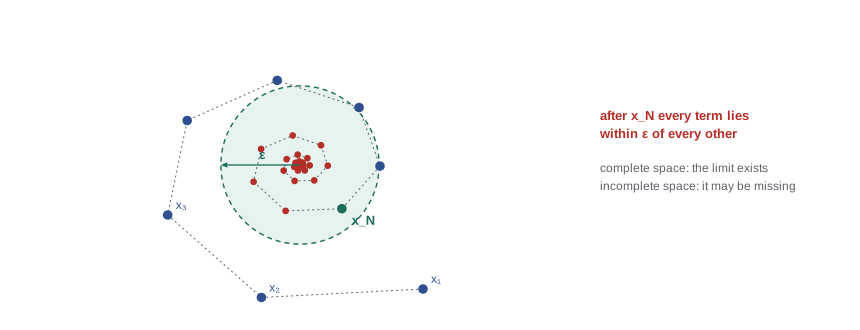
Definition. A sequence \((x_n)\) in a metric space \((X, d)\) is Cauchy if for every \(\varepsilon > 0\) there is an \(N\) with \(d(x_m, x_n) < \varepsilon\) for all \(m, n \ge N\). The space is complete if every Cauchy sequence in \(X\) converges to a point of \(X\).

Every convergent sequence is Cauchy, by the triangle inequality: if \(x_n \to x\), then \(d(x_m, x_n) \le d(x_m, x) + d(x, x_n)\). The converse is the content of completeness, and it can fail. In \(\mathbb{Q}\), the decimal approximations \(1, 1.4, 1.41, 1.414, \dots\) of \(\sqrt{2}\) form a Cauchy sequence with no rational limit. In the space \((0, 1)\) with the usual distance, \(\frac{1}{n}\) is Cauchy but its limit 0 is missing. Completeness is a property of the metric space, not of the set alone: \((0, 1)\) and \(\mathbb{R}\) are in one-to-one correspondence by continuous maps in both directions, but one is complete and the other is not.

Theorem 8.1. \(\mathbb{R}^n\) is complete with each of the metrics \(d_1\), \(d_2\), \(d_\infty\).

Proof. By the inequalities of lesson 7, a sequence is Cauchy, or convergent, in one of these metrics if and only if it is in the others, so it suffices to treat \(d_\infty\). If \((x^{(k)})\) is Cauchy in \(d_\infty\), then for each coordinate \(i\), \(|x_i^{(k)} - x_i^{(l)}| \le d_\infty(x^{(k)}, x^{(l)})\), so the real sequence \((x_i^{(k)})_k\) is Cauchy and converges to some \(x_i\), by completeness of \(\mathbb{R}\). Given \(\varepsilon > 0\), choose for each of the \(n\) coordinates a \(K_i\) with \(|x_i^{(k)} - x_i| < \varepsilon\) for \(k \ge K_i\), and let \(K = \max K_i\). Then \(d_\infty(x^{(k)}, x) < \varepsilon\) for \(k \ge K\). \(\square\)

Theorem 8.2. A subset \(Y\) of a complete metric space \(X\) is complete, with the inherited metric, if and only if it is closed in \(X\).

Proof. If \(Y\) is closed and \((y_n)\) is Cauchy in \(Y\), it converges in \(X\) to some \(x\), and \(x \in Y\) by theorem 7.6. If \(Y\) is complete and \(y_n \in Y\) converges in \(X\) to \(x\), then \((y_n)\) is Cauchy, so it converges in \(Y\) to some \(y\); by uniqueness of limits in \(X\), \(x = y \in Y\). So \(Y\) is closed. \(\square\)

Completeness of spaces of functions

Theorem 8.3. The space \(C[a, b]\) with the sup metric is complete.

Proof. A Cauchy sequence \((f_n)\) in the sup metric is exactly a uniformly Cauchy sequence. By theorem 2.2 it converges uniformly to some function \(f\) on \([a, b]\), and by the uniform limit theorem, theorem 3.1, \(f\) is continuous. So \(f \in C[a, b]\) and \(d_\infty(f_n, f) \to 0\). \(\square\)

Theorem 8.4. The space \(C[0, 1]\) with the integral metric \(d_1(f, g) = \int_0^1 |f - g|\) is not complete.

Proof. Let \(f_n\) be 0 on \([0, \frac{1}{2}]\), rise linearly from 0 to 1 on \([\frac{1}{2}, \frac{1}{2} + \frac{1}{n}]\), and be 1 on \([\frac{1}{2} + \frac{1}{n}, 1]\), for \(n \ge 2\). For \(m > n\), \(f_m\) and \(f_n\) differ only on \([\frac{1}{2}, \frac{1}{2} + \frac{1}{n}]\), where both lie in \([0, 1]\), so \(d_1(f_m, f_n) \le \frac{1}{n}\), and the sequence is Cauchy. Suppose \(d_1(f_n, f) \to 0\) for some continuous \(f\). Since \(f_n = 0\) on \([0, \frac{1}{2}]\), \(\int_0^{1/2} |f| \le d_1(f_n, f) \to 0\), so \(f = 0\) on \([0, \frac{1}{2}]\). For any \(c > \frac{1}{2}\), once \(\frac{1}{2} + \frac{1}{n} < c\) we have \(f_n = 1\) on \([c, 1]\), so \(\int_c^1 |f - 1| \le d_1(f_n, f) \to 0\) and \(f = 1\) on \([c, 1]\). Hence \(f = 1\) on \((\frac{1}{2}, 1]\) and \(f(\frac{1}{2}) = 0\), contradicting continuity. \(\square\)

The sequence 'wants' to converge to a step function, which is not in the space. Completing \(C[0, 1]\) in the integral metric produces the space \(L^1[0, 1]\) of Lebesgue integrable functions, one of the main objects of MATH-441. The code below makes the contrast concrete.

import math

def dsup(f, g, pts=4097):
    return max(abs(f(i / (pts - 1)) - g(i / (pts - 1))) for i in range(pts))

def dint(f, g, m=20000):
    h = 1 / m                                   # midpoint rule for the integral of |f - g|
    return h * sum(abs(f((i + 0.5) * h) - g((i + 0.5) * h)) for i in range(m))

# 1. partial sums of e^x are Cauchy in the sup metric, and the limit e^x is in C[0, 1]
s = lambda n: (lambda x: sum(x ** k / math.factorial(k) for k in range(n + 1)))
print(" n   d_sup(s_n, s_2n)   d_sup(s_n, e^x)")
for n in [2, 4, 8, 16]:
    print(f"{n:2d}   {dsup(s(n), s(2 * n)):14.3e}   {dsup(s(n), math.exp):14.3e}")

# 2. ramps: Cauchy in the integral metric, not in the sup metric, no continuous limit
ramp = lambda n: (lambda x: min(1.0, max(0.0, n * (x - 0.5))))
print()
print("  n   d_int(f_n, f_2n)   d_sup(f_n, f_2n)")
for n in [4, 16, 64, 256]:
    print(f"{n:4d}   {dint(ramp(n), ramp(2 * n)):12.6f}   {dsup(ramp(n), ramp(2 * n)):14.4f}")

 n   d_sup(s_n, s_2n)   d_sup(s_n, e^x)
 2        2.083e-01        2.183e-01
 4        9.945e-03        9.948e-03
 8        3.059e-06        3.059e-06
16        3.109e-15        3.109e-15

  n   d_int(f_n, f_2n)   d_sup(f_n, f_2n)
   4       0.062500           0.5000
  16       0.015625           0.5000
  64       0.003906           0.5000
 256       0.000977           0.5000

The partial sums of the exponential series are Cauchy in the sup metric, and their sup distance to \(e^x\) shrinks rapidly, as theorem 8.3 predicts. The ramps have integral distance \(\frac{1}{4n}\) from their successors, which tends to 0, while the sup distance stays at \(\frac{1}{2}\), attained at \(x = \frac{1}{2} + \frac{1}{2n}\): they are Cauchy in one metric but not the other, and in the integral metric there is no continuous function for them to converge to.

Compactness

Definition. An open cover of a subset \(K\) of a metric space is a collection of open sets whose union contains \(K\). The set \(K\) is compact if every open cover of \(K\) has a finite subcover, that is, finitely many of the sets already cover \(K\). It is sequentially compact if every sequence in \(K\) has a subsequence converging to a point of \(K\).

In MATH-241 compactness of a subset of \(\mathbb{R}\) was defined by sequences. The open cover definition, which goes back to Émile Borel's 1895 work on covering \([a, b]\) by countably many intervals, generalizes to topological spaces where sequences are not enough. In metric spaces the two agree.

Theorem 8.5. A metric space is compact if and only if it is sequentially compact.

Proof that compact implies sequentially compact. Let \((x_n)\) be a sequence with no convergent subsequence. Then every point \(p\) has a ball \(B(p, r_p)\) containing \(x_n\) for only finitely many indices \(n\). Otherwise, for some \(p\), every ball \(B(p, \frac{1}{k})\) contains \(x_n\) for infinitely many \(n\), and we could choose \(n_1 < n_2 < \dots\) with \(x_{n_k} \in B(p, \frac{1}{k})\), a subsequence converging to \(p\). The balls \(B(p, r_p)\) cover the space; by compactness finitely many do. But then only finitely many indices \(n\) occur in total, which is absurd.

Proof that sequentially compact implies compact. We need two lemmas about a sequentially compact space \(X\).

Lemma A (Lebesgue number). For every open cover \(\{U_\alpha\}\) of \(X\) there is \(\delta > 0\) such that every ball \(B(x, \delta)\) lies inside some single \(U_\alpha\). Proof. If not, for each \(n\) there is \(x_n\) such that \(B(x_n, \frac{1}{n})\) lies in no \(U_\alpha\). A subsequence \(x_{n_k}\) converges to some \(x\), which lies in some \(U_\alpha\), with \(B(x, \varepsilon) \subseteq U_\alpha\). Choose \(k\) with \(d(x_{n_k}, x) < \frac{\varepsilon}{2}\) and \(\frac{1}{n_k} < \frac{\varepsilon}{2}\). Then \(B(x_{n_k}, \frac{1}{n_k}) \subseteq B(x, \varepsilon) \subseteq U_\alpha\), a contradiction.

Lemma B (total boundedness). For every \(\delta > 0\), finitely many balls of radius \(\delta\) cover \(X\). Proof. If not, choose \(x_1\) arbitrarily and, inductively, \(x_{n+1}\) outside \(B(x_1, \delta) \cup \dots \cup B(x_n, \delta)\). Then \(d(x_i, x_j) \ge \delta\) for all \(i \ne j\), so no subsequence is Cauchy and none converges, a contradiction.

Now let \(\{U_\alpha\}\) be an open cover, take \(\delta\) from lemma A, and cover \(X\) by finitely many balls \(B(x_1, \delta), \dots, B(x_m, \delta)\) using lemma B. Each \(B(x_i, \delta)\) lies in some \(U_{\alpha_i}\), so \(U_{\alpha_1}, \dots, U_{\alpha_m}\) cover \(X\). \(\square\)

Theorem 8.6. A compact subset \(K\) of a metric space is closed and bounded.

Proof. The balls \(B(p, n)\), \(n = 1, 2, \dots\), for a fixed \(p\) cover \(K\); a finite subcover shows \(K \subseteq B(p, N)\), so \(K\) is bounded. If \(x_n \in K\) and \(x_n \to x\), every subsequence also converges to \(x\), and sequential compactness gives a subsequence with limit in \(K\), so \(x \in K\), and \(K\) is closed. \(\square\)

Theorem 8.7 (Heine–Borel). A subset of \(\mathbb{R}^n\) is compact if and only if it is closed and bounded.

Proof. One direction is theorem 8.6. Conversely let \(K\) be closed and bounded and \((x^{(k)})\) a sequence in \(K\). Its first coordinates form a bounded real sequence, which by the Bolzano–Weierstrass theorem has a convergent subsequence. Passing to that subsequence, the second coordinates have a convergent subsequence, and so on; after \(n\) steps we have a subsequence along which every coordinate converges, so it converges in \(\mathbb{R}^n\), and its limit lies in \(K\) because \(K\) is closed. So \(K\) is sequentially compact, hence compact. \(\square\)

In \(C[0, 1]\) with the sup metric, closed and bounded is not enough. Let \(g_n\) be a tent of height 1 supported on \([\frac{1}{n + 1}, \frac{1}{n}]\). The supports do not overlap, so \(d_\infty(g_m, g_n) = 1\) for \(m \ne n\), and no subsequence is Cauchy. The closed unit ball \(\{f : d_\infty(f, 0) \le 1\}\) is closed and bounded but not compact. Lesson 9 describes the compact subsets of \(C[a, b]\) by the Arzelà–Ascoli theorem.

The contraction mapping theorem

Definition. A map \(T: X \to X\) on a metric space is a contraction if there is a constant \(q < 1\) with \(d(Tx, Ty) \le q\,d(x, y)\) for all \(x, y \in X\). A point with \(Tx = x\) is a fixed point.

Theorem 8.8 (Banach fixed point theorem). Let \((X, d)\) be a nonempty complete metric space and \(T: X \to X\) a contraction with constant \(q < 1\). Then \(T\) has exactly one fixed point \(x^*\). For any starting point \(x_0\), the iterates \(x_{n+1} = Tx_n\) converge to \(x^*\), with \[d(x_n, x^*) \le \frac{q^n}{1 - q}\,d(x_1, x_0) \quad \text{and} \quad d(x_n, x^*) \le \frac{q}{1 - q}\,d(x_n, x_{n-1}).\]

Proof. By induction \(d(x_{k+1}, x_k) \le q^k d(x_1, x_0)\). For \(m > n\), the triangle inequality and the geometric series give \[d(x_m, x_n) \le \sum_{k=n}^{m-1} d(x_{k+1}, x_k) \le d(x_1, x_0)\sum_{k=n}^{m-1} q^k < \frac{q^n}{1 - q}\,d(x_1, x_0).\] The right side tends to 0, so \((x_n)\) is Cauchy, and by completeness it converges to some \(x^*\). A contraction is continuous, since \(d(Tx, Ty) \le q\,d(x, y)\), so \(Tx^* = \lim Tx_n = \lim x_{n+1} = x^*\). If \(Ty = y\) as well, then \(d(x^*, y) = d(Tx^*, Ty) \le q\,d(x^*, y)\), which forces \(d(x^*, y) = 0\). Letting \(m \to \infty\) in the displayed inequality gives the first error bound; applying it with \(x_{n-1}\) as the starting point gives the second. \(\square\)

Stefan Banach proved the theorem in his doctoral thesis, published in Fundamenta Mathematicae in 1922, in the setting of complete normed spaces, now called Banach spaces. The method of successive approximations behind it is much older: Joseph Liouville used it for differential equations in the 1830s and Émile Picard systematized it in 1890. Banach's contribution was to isolate the two ingredients, a contraction and a complete space, that make the method work.

All three hypotheses are needed. On the incomplete space \((0, 1]\), \(Tx = \frac{x}{2}\) is a contraction with no fixed point. On \(\mathbb{R}\), \(Tx = x + 1\) satisfies \(d(Tx, Ty) = d(x, y)\), with \(q = 1\), and has no fixed point. And \(Tx = x + \frac{1}{x}\) on \([1, \infty)\) satisfies \(|Tx - Ty| < |x - y|\) for \(x \ne y\), but not with a constant \(q < 1\), and has no fixed point.

On an interval the mean value theorem gives an easy test. If \(g\) maps a closed interval \(I\) into itself and \(|g^\prime(x)| \le q < 1\) on \(I\), then \(|g(x) - g(y)| = |g^\prime(\xi)||x - y| \le q|x - y|\), so \(g\) is a contraction of the complete space \(I\).

import math

def iterate(T, x0, q, n):
    xs = [x0]
    for _ in range(n):
        xs.append(T(xs[-1]))
    return xs

# 1. T(x) = cos x on [0, 1]: maps [0, 1] into [cos 1, 1] and |T'(x)| = |sin x| <= sin 1 < 1
q = math.sin(1)
xs = iterate(math.cos, 0.0, q, 30)
star = 0.7390851332151607          # the fixed point (Dottie number), to 16 digits
print(f"q = sin 1 = {q:.4f}")
print(" n     x_n          actual error    a priori bound")
for n in [1, 5, 10, 20, 30]:
    bound = q ** n / (1 - q) * abs(xs[1] - xs[0])
    print(f"{n:2d}   {xs[n]:.10f}   {abs(xs[n] - star):12.3e}   {bound:12.3e}")

# 2. Newton's method for sqrt 2 as a contraction: N(x) = (x + 2/x)/2 maps [1, 2] into [sqrt 2, 1.5]
#    and N'(x) = 1/2 - 1/x^2 lies in [-1/2, 1/4] there, so q = 1/2
N = lambda x: (x + 2 / x) / 2
ys = iterate(N, 2.0, 0.5, 5)
print()
print(" n     y_n                 actual error   a priori bound (q = 1/2)")
for n, y in enumerate(ys):
    bound = 0.5 ** n / 0.5 * abs(ys[1] - ys[0])
    print(f"{n:2d}   {y:.15f}   {abs(y - math.sqrt(2)):10.2e}     {bound:10.2e}")

q = sin 1 = 0.8415
 n     x_n          actual error    a priori bound
 1   1.0000000000      2.609e-01      5.308e+00
 5   0.7934803587      5.440e-02      2.661e+00
10   0.7314040424      7.681e-03      1.123e+00
20   0.7389377567      1.474e-04      1.998e-01
30   0.7390822985      2.835e-06      3.557e-02

 n     y_n                 actual error   a priori bound (q = 1/2)
 0   2.000000000000000     5.86e-01       1.00e+00
 1   1.500000000000000     8.58e-02       5.00e-01
 2   1.416666666666667     2.45e-03       2.50e-01
 3   1.414215686274510     2.12e-06       1.25e-01
 4   1.414213562374690     1.59e-12       6.25e-02
 5   1.414213562373095     2.22e-16       3.12e-02

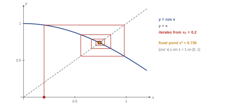
For \(\cos x\) the actual error shrinks by a factor of about \(\sin(0.739) \approx 0.67\) per step, a little better than the guaranteed \(q = \sin 1 \approx 0.84\), and always stays below the a priori bound. For Newton's method the contraction estimate with \(q = \frac{1}{2}\) is valid but very pessimistic: near the fixed point \(N^\prime(\sqrt{2}) = 0\), so the true contraction factor tends to 0 and the number of correct digits roughly doubles each step.