From numbers to functions: why convergence of functions matters

Real Analysis I was about numbers. A sequence \((a_n)\) of real numbers converges to \(a\) if for every \(\varepsilon > 0\) there is an \(N\) with \(|a_n - a| < \varepsilon\) for all \(n \ge N\). On that single definition, together with the completeness of the real line, we built limits of functions, continuity, the derivative and the Riemann integral. Real Analysis II asks the next question: what does it mean for a sequence of functions to converge, and which properties survive the passage to the limit?

The question is not academic. Most of the functions that matter in mathematics and physics are not given by a closed formula. They are given as limits: the sum of a power series, the sum of a Fourier series, the solution of a differential equation obtained by repeated approximation, the limit of a numerical method as the step size shrinks. To know that such a limit is continuous, or that it can be differentiated or integrated term by term, we need theorems about limits of functions, and those theorems turn out to need a stronger notion of convergence than the obvious one.

Functions defined as limits

Here are four functions that are best understood as limits of simpler ones.

• The exponential function \(e^x = \sum_{k=0}^{\infty} \frac{x^k}{k!}\) is the limit of the polynomials \(p_n(x) = \sum_{k=0}^{n} \frac{x^k}{k!}\). We would like to prove that \(\frac{d}{dx} e^x = e^x\) by differentiating the series term by term.

• The square wave, equal to 1 on \((0, \pi)\) and \(-1\) on \((-\pi, 0)\), is the sum of its Fourier series \(\frac{4}{\pi}\sum_{k \text{ odd}} \frac{\sin kx}{k}\). Every partial sum is a smooth function, yet the limit jumps.

• The solution of \(y' = y\), \(y(0) = 1\), can be produced by Picard iteration: start with \(y_0(x) = 1\) and set \(y_{n+1}(x) = 1 + \int_0^x y_n(t)\,dt\). The iterates are exactly the polynomials \(p_n\) above, and their limit solves the equation.

• Weierstrass's continuous, nowhere differentiable function \(W(x) = \sum_{k=0}^{\infty} a^k \cos(b^k \pi x)\) is a limit of smooth functions that has no derivative anywhere.

The first and third examples behave as we hope. The second and fourth show that smoothness can be lost in the limit, and the second even loses continuity. The task of the first half of this course is to understand exactly what goes wrong and to find conditions under which nothing does.

Pointwise limits can misbehave

The obvious way to define the limit of a sequence of functions \(f_n: A \to \mathbb{R}\) is point by point: \(f_n \to f\) pointwise if \(f_n(x) \to f(x)\) for every \(x \in A\). That is, for every \(x\) and every \(\varepsilon > 0\) there is an \(N\), which may depend on both \(x\) and \(\varepsilon\), such that \(|f_n(x) - f(x)| < \varepsilon\) for \(n \ge N\). The definition is natural, but pointwise limits are badly behaved.

Continuity can be lost. On \([0, 1]\) let \(f_n(x) = x^n\). For \(0 \le x < 1\), \(x^n \to 0\), while \(f_n(1) = 1\) for every \(n\). The pointwise limit is \(f(x) = 0\) for \(x < 1\) and \(f(1) = 1\), which is discontinuous at 1, although every \(f_n\) is a polynomial.

Integrals can be lost. Let \(g_n\) be the tent function on \([0, 1]\) that rises linearly from 0 at \(x = 0\) to height \(n\) at \(x = \frac{1}{n}\), falls back to 0 at \(x = \frac{2}{n}\), and is 0 on \([\frac{2}{n}, 1]\). Each \(g_n\) is continuous with \(\int_0^1 g_n = 1\), the area of a triangle with base \(\frac{2}{n}\) and height \(n\). Yet \(g_n(x) \to 0\) for every \(x\): at \(x = 0\) every value is 0, and for \(x > 0\) we have \(g_n(x) = 0\) as soon as \(\frac{2}{n} < x\). So \(\lim \int_0^1 g_n = 1\) while \(\int_0^1 \lim g_n = 0\).

Derivatives can be lost. Let \(h_n(x) = \frac{\sin(n^2 x)}{n}\). Then \(|h_n(x)| \le \frac{1}{n}\), so \(h_n \to 0\) at every point, and in fact uniformly, in the sense of lesson 2. But \(h_n'(x) = n\cos(n^2 x)\), and at \(x = 0\) this is \(n \to \infty\). The derivatives of the approximating functions do not converge to the derivative of the limit.

In each case the trouble is an interchange of two limiting processes. Continuity of the limit at \(x_0\) asks whether \(\lim_{x \to x_0} \lim_{n \to \infty} f_n(x) = \lim_{n \to \infty} \lim_{x \to x_0} f_n(x)\). Integrating the limit asks whether the limit of integrals equals the integral of the limit, and an integral is itself a limit of Riemann sums. Differentiating asks whether two limits, one in \(n\) and one in the difference quotient, commute. Limits do not commute in general. For the double sequence \(a_{m,n} = \frac{m}{m + n}\) we have \(\lim_m \lim_n a_{m,n} = 0\) but \(\lim_n \lim_m a_{m,n} = 1\).

A famous error and its correction

In his Cours d'analyse of 1821, Augustin-Louis Cauchy stated as a theorem that the sum of a convergent series of continuous functions is continuous. His argument went roughly as follows: if \(s(x) = s_n(x) + r_n(x)\), where \(s_n\) is the partial sum and \(r_n\) the remainder, then \(s_n\) is continuous and \(r_n(x)\) is small for large \(n\), so \(s\) changes little when \(x\) changes little. The flaw is that \(r_n(x)\) is small for large \(n\) at each fixed \(x\), but how large \(n\) must be may depend on \(x\), and near a bad point it may have to grow without bound.

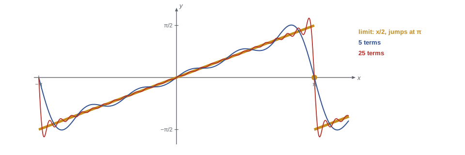
In 1826 the Norwegian mathematician Niels Henrik Abel, in a paper on the binomial series published in the first volume of Crelle's Journal, remarked in a footnote that Cauchy's theorem 'seems to admit exceptions'. His example was the series \[\sin x - \frac{\sin 2x}{2} + \frac{\sin 3x}{3} - \dots = \sum_{k=1}^{\infty} (-1)^{k+1}\frac{\sin kx}{k},\] which converges for every \(x\) to \(\frac{x}{2}\) when \(-\pi < x < \pi\), and to 0 at \(x = \pm\pi\). Extended periodically, its sum jumps by \(\pi\) at every odd multiple of \(\pi\). Every term is continuous; the sum is not.

Abel's example was a Fourier series, and Fourier's work of 1807 to 1822 had already produced many series of continuous functions with discontinuous sums. The resolution came slowly. In 1847 and 1848 Philipp Ludwig von Seidel and George Gabriel Stokes independently identified the phenomenon of convergence that becomes arbitrarily slow near a point. Karl Weierstrass used the condition we now call uniform convergence, in German gleichmäßige Konvergenz, in a manuscript of 1841 on power series that was not published until 1894, and he made it central to analysis in his Berlin lectures of the 1860s; notes of his 1861 lectures contain the definition and the theorem that uniform limits of continuous functions are continuous. Cauchy himself added a corrected hypothesis, close to uniform convergence, in 1853.

Uniform convergence asks for a single \(N\) that works for every \(x\) at once. Lesson 2 gives the precise definition and lesson 3 proves that it rescues continuity and integration, and, with an extra hypothesis, differentiation.

Seeing the slow convergence

The code below evaluates partial sums of Abel's series near \(x = \pi\). Far from \(\pi\) the partial sums settle quickly to \(\frac{x}{2}\); close to \(\pi\) many more terms are needed, and at \(x = \pi\) itself every partial sum is 0.

import math

def S(N, x):
    """Partial sum of Abel's series sin x - sin 2x/2 + sin 3x/3 - ..."""
    return sum((-1) ** (k + 1) * math.sin(k * x) / k for k in range(1, N + 1))

print("   x        x/2      N=10      N=100     N=1000")
for x in [1.0, 2.5, 3.0, 3.1, 3.14, math.pi]:
    row = [S(N, x) for N in (10, 100, 1000)]
    print(f"{x:7.4f}  {x / 2:7.4f}  " + "  ".join(f"{v:8.4f}" for v in row))

# how many terms until the error stays below 0.01 (checked up to 20000 terms)?
for x in [1.0, 3.0, 3.1, 3.13]:
    s, last_bad = 0.0, 0
    for N in range(1, 20001):
        s += (-1) ** (N + 1) * math.sin(N * x) / N
        if abs(s - x / 2) >= 0.01:
            last_bad = N
    print(f"x = {x}: error below 0.01 from N = {last_bad + 1} on")

   x        x/2      N=10      N=100     N=1000
 1.0000   0.5000    0.5482    0.5002    0.4994
 2.5000   1.2500    1.1106    1.2510    1.2492
 3.0000   1.5000    1.2454    1.5017    1.5068
 3.1000   1.5500    0.4113    1.7017    1.5676
 3.1400   1.5700    0.0159    0.1590    1.3843
 3.1416   1.5708    0.0000    0.0000    0.0000
x = 1.0: error below 0.01 from N = 52 on
x = 3.0: error below 0.01 from N = 689 on
x = 3.1: error below 0.01 from N = 2347 on
x = 3.13: error below 0.01 from N = 8421 on

The pattern in the output is the whole story of this course's first half. At every fixed \(x\) the partial sums converge, but the number of terms needed for a given accuracy is unbounded as \(x \to \pi\). There is no single \(N\) that works on the whole interval \((-\pi, \pi)\), and that is exactly why the limit can jump at \(\pi\) even though every partial sum is continuous there.

Functions as points

A second idea runs through the course. Instead of thinking of a sequence of functions as many sequences of numbers, one for each \(x\), we can think of each function as a single point in a space of functions and measure the distance between two functions by one number. For bounded functions on a set \(A\) the natural choice is the supremum distance \[d_\infty(f, g) = \sup_{x \in A} |f(x) - g(x)|,\] the largest vertical gap between the graphs. With this distance, \(f_n \to f\) uniformly exactly when \(d_\infty(f_n, f) \to 0\), so uniform convergence is ordinary convergence of points in a space whose points are functions.

This point of view, developed by Vito Volterra, David Hilbert, Maurice Fréchet and others around 1900, led Fréchet in his thesis of 1906 to define abstract metric spaces: sets with a distance satisfying a few axioms. Lessons 7 to 9 develop metric spaces and show that the definitions of Real Analysis I, such as Cauchy sequences, completeness, compactness and continuity, make sense in any of them. One theorem proved there, the contraction mapping theorem of Stefan Banach's 1922 thesis, is the engine behind the last third of the course.

Several variables

The final part of the course turns to functions \(f: \mathbb{R}^n \to \mathbb{R}^m\). The derivative of such a function at a point is not a number but a linear map, the best linear approximation to \(f\) near that point. Once this is understood, the inverse function theorem says that a continuously differentiable map whose derivative is invertible at a point is itself invertible near that point, and the implicit function theorem says when an equation \(F(x, y) = 0\) can be solved for \(y\) as a function of \(x\). Both are proved by iteration, using the contraction mapping theorem in the complete metric space \(\mathbb{R}^n\). Their applications include changes of variables, the description of curves and surfaces by equations, and the method of Lagrange multipliers.

The course therefore follows one thread. We start with a concrete problem, the failure of pointwise limits; we solve it with uniform convergence, which is convergence in the sup metric; we abstract to metric spaces, where completeness gives the contraction mapping theorem; and we apply that theorem to solve nonlinear equations in several variables.

What carries over from Real Analysis I

We will use freely the results of MATH-241: the least upper bound property, the Bolzano–Weierstrass theorem, the Cauchy criterion for sequences and series, the comparison, ratio and root tests, the extreme value theorem and the Heine–Cantor theorem on uniform continuity, the mean value theorem and Taylor's theorem, and the Riemann integral with the fundamental theorem of calculus. Two of these deserve a reminder because they are close cousins of the new ideas.

Uniform continuity of \(f\) on \(A\) asks for one \(\delta\) that works at every point, just as uniform convergence asks for one \(N\) that works at every point. In both definitions the quantifier 'for all \(x\)' moves from the front of the sentence to the end. Compare: \(f\) is continuous on \(A\) if for every \(x \in A\) and \(\varepsilon > 0\) there is a \(\delta > 0\) such that \(|y - x| < \delta\) implies \(|f(y) - f(x)| < \varepsilon\); \(f\) is uniformly continuous if for every \(\varepsilon > 0\) there is a \(\delta > 0\) such that for all \(x, y \in A\), \(|y - x| < \delta\) implies \(|f(y) - f(x)| < \varepsilon\). Exactly the same move turns pointwise convergence into uniform convergence.

The Cauchy criterion says a sequence of reals converges if and only if its terms eventually stay close to each other. Its importance is that it decides convergence without knowing the limit. We will prove a uniform Cauchy criterion for sequences of functions in lesson 2 and use it to prove the Weierstrass M-test in lesson 4; in lesson 8 the same idea becomes the definition of a complete metric space.

How the course is organized

Lessons 2 to 6 treat sequences and series of functions: pointwise and uniform convergence (lesson 2), the theorems on continuity, integration and differentiation of limits (lesson 3), series and the Weierstrass M-test (lesson 4), power series and Abel's theorem (lesson 5), and the Weierstrass approximation theorem, which says every continuous function on a closed interval is a uniform limit of polynomials (lesson 6). Lessons 7 to 9 develop metric spaces: open and closed sets (lesson 7), completeness, compactness and the contraction mapping theorem (lesson 8), and continuity with an overview of the Arzelà–Ascoli theorem (lesson 9). Lessons 10 to 12 treat differentiation in \(\mathbb{R}^n\), the inverse function theorem and the implicit function theorem.

Measure theory and the Lebesgue integral, which handle limits of integrals far more flexibly than the Riemann integral, are the subject of MATH-441. General topological spaces, which abstract the notion of open set beyond distances, belong to MATH-447, and manifolds, the natural home of the implicit function theorem, to MATH-430. This course provides the foundations each of them needs.