
MATH-300 · Lesson 4 of 5 · 29 min
Interpolation and curve fitting
Engineers constantly work with functions known only at discrete points: properties in a steam table, a pump's head at tested flow rates, survey elevations along a road, sensor readings every second. Two tasks follow. Interpolation finds values between exact data points, with a curve that passes through every one of them. Curve fitting finds a simple formula that follows noisy data closely without passing through each point. Choosing the right one, and the right curve, is the subject of this chapter.
Linear interpolation
The simplest interpolant joins neighbouring points with straight lines. Between \((x_0, y_0)\) and \((x_1, y_1)\):
Every engineering student does this with property tables. Its error is about \(\frac{1}{8}h^2|f''|\) for spacing h, small when the function is nearly straight over the interval and larger where it curves.
Worked problem
Saturation pressure from a steam table
A steam table gives the saturation pressure of water as 101.42 kPa at 100 °C and 143.38 kPa at 110 °C. Estimate it at 105 °C by linear interpolation. (The IAPWS-IF97 value is 120.90 kPa.)
Show solution
- \(P = 101.42 + \dfrac{143.38 - 101.42}{10}(5) = 101.42 + 20.98 = 122.40\) kPa.
- Error: \(122.40 - 120.90 = 1.50\) kPa, or 1.2%.
Answer: 122.4 kPa, 1.2% high, because the pressure curve bends upward (it is convex, so the chord lies above it). Tables with closer spacing, or a higher-degree interpolant, reduce the error
Polynomial interpolation
Through n + 1 points with distinct x values there is exactly one polynomial of degree at most n. Two convenient ways to write it:
- Lagrange form: \(p(x) = \sum_i y_i L_i(x)\), where each basis polynomial \(L_i(x) = \prod_{j \ne i}\frac{x - x_j}{x_i - x_j}\) equals 1 at \(x_i\) and 0 at the other nodes. Elegant for theory.
- Newton form with divided differences: \(p(x) = f[x_0] + f[x_0, x_1](x - x_0) + f[x_0, x_1, x_2](x - x_0)(x - x_1) + \cdots\). Adding a point adds one term, without recomputing the others. Better for hand and computer work.
Divided differences are computed in a table: \(f[x_i, x_{i+1}] = \dfrac{f[x_{i+1}] - f[x_i]}{x_{i+1} - x_i}\), and each higher difference is the difference of the two below it divided by the span of x values involved.
Worked problem
Quadratic interpolation in the steam table
Add the point (120 °C, 198.67 kPa) and interpolate quadratically at 105 °C and 115 °C. (IF97 values: 120.90 and 169.18 kPa.)
Show solution
- First differences: \(f[100, 110] = 41.96/10 = 4.1958\); \(f[110, 120] = 55.29/10 = 5.5289\).
- Second difference: \(f[100, 110, 120] = (5.5289 - 4.1958)/20 = 0.066655\).
- \(p(105) = 101.42 + 4.1958(5) + 0.066655(5)(-5) = 120.73\) kPa (error −0.14%).
- \(p(115) = 101.42 + 4.1958(15) + 0.066655(15)(5) = 169.35\) kPa (error +0.10%). Linear interpolation gives 171.02 kPa (+1.1%).
Answer: The quadratic term, which captures the curvature, cuts the error about tenfold: 120.73 and 169.35 kPa
The danger of high degree: Runge's phenomenon
It is tempting to think more points and a higher degree always help. They do not. The error of polynomial interpolation is
and with equally spaced points the product term becomes huge near the ends of the interval. For the smooth function \(f(x) = 1/(1 + 25x^2)\) on [−1, 1], a degree-10 polynomial through 11 equally spaced points has a maximum error of 1.92, far larger than the function itself, and the error grows as the degree increases.
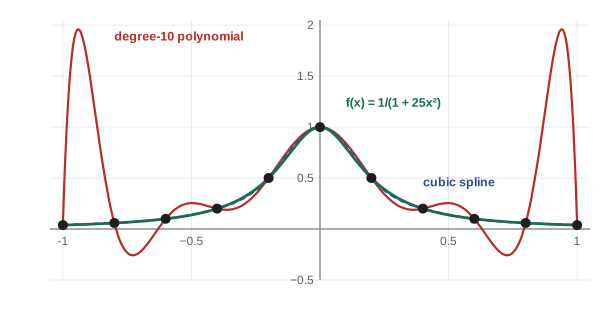
Two cures: cluster the points toward the ends (Chebyshev nodes \(x_k = \cos\frac{(2k + 1)\pi}{2(n + 1)}\) reduce the degree-10 error to 0.11), or, far more common in engineering, use piecewise polynomials of low degree.
Cubic splines
A cubic spline uses a separate cubic between each pair of adjacent points, chosen so that the curve and its first and second derivatives are continuous at every interior point. The result is smooth to the eye and to the touch, like the flexible strips of wood (splines) that shipwrights and draftsmen once bent through pegs to draw hull lines.
The continuity conditions give a tridiagonal linear system for the second derivatives at the nodes (Lesson 3), solved in O(n) operations. Two end conditions complete it: natural (zero second derivative at the ends), clamped (specified end slopes) or not-a-knot (the default in many libraries).
Through the same 11 points as above, a cubic spline has maximum error 0.022 for the Runge function, almost 100 times better than the degree-10 polynomial. Splines are used for road and railway alignments, cam profiles, CAD curves and surfaces, robot trajectories and smooth interpolation of tabulated data.
Least-squares curve fitting
Measured data contain noise, so a curve through every point would chase the noise. Instead, choose a simple model with a few parameters and fit it by least squares: minimize the sum of squared residuals \(\sum (y_i - \hat{y}_i)^2\), as in STAT-235's straight-line regression.
For a polynomial model \(y = c_0 + c_1x + \cdots + c_mx^m\) with m much smaller than the number of points, the fit is a linear least-squares problem \(V\mathbf{c} \approx \mathbf{y}\), where V is the matrix whose columns are \(1, x, x^2, \ldots\). It can be solved through the normal equations \(V^TV\mathbf{c} = V^T\mathbf{y}\), but \(V^TV\) squares the condition number of V (Lesson 3), so libraries use the more stable QR factorization instead (np.polyfit, np.linalg.lstsq, MATLAB polyfit).
Worked problem
Fitting a pump curve
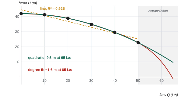
A centrifugal pump test gives head H (m) at flow Q (L/s): (0, 42.0), (10, 41.2), (20, 38.9), (30, 34.8), (40, 29.6), (50, 22.7). Fit a straight line and a quadratic, and estimate the head at 35 L/s.
Show solution
- Line: \(H = 44.54 - 0.387Q\), R² = 0.925. Its residuals run −2.5, +0.5, +2.1, +1.9, +0.5, −2.5: a clear curved pattern, so the form is wrong.
- Quadratic: \(H = 42.03 - 0.0110Q - 0.00752Q^2\), R² = 0.9999, with residuals of at most 0.14 m and no pattern.
- At 35 L/s: \(H = 42.03 - 0.0110(35) - 0.00752(35)^2 = 32.4\) m.
Answer: Use the quadratic: H(35) = 32.4 m. Pump curves are physically close to quadratic in flow, which is why this simple model fits so well
Overfitting
A degree-5 polynomial passes exactly through all six pump points (R² = 1). Inside the data range it differs from the quadratic by only a few centimetres, but beyond it the two separate fast: at 65 L/s the quadratic predicts 9.6 m of head, while the degree-5 curve predicts −1.6 m, which is physically impossible. Extra parameters fit the noise, not the physics. Choose the simplest model that leaves residuals without a pattern, prefer models with a physical basis, and never trust extrapolation of a high-degree fit.
Nonlinear models
Many physical laws are not polynomials: exponential decay, power laws, saturation curves. Two approaches:
- Linearize when possible: \(y = ae^{bx}\) becomes \(\ln y = \ln a + bx\); \(y = ax^b\) becomes \(\ln y = \ln a + b\ln x\). Fit a line to the transformed data. Quick, but it weights the errors differently from the original scale.
- Nonlinear least squares: minimize the squared residuals in the original form directly, iteratively (Gauss–Newton or Levenberg–Marquardt, scipy.optimize.curve_fit). It needs reasonable starting values and returns parameter uncertainties too.
Worked problem
Biochemical oxygen demand
The BOD of a wastewater sample (mg/L) measured on days 1 to 7 is 48.8, 91.5, 131.3, 153.0, 164.3, 187.1, 197.5. Fit the first-order model \(y = L_0(1 - e^{-kt})\), where L₀ is the ultimate BOD and k the rate constant.
Show solution
- The model is nonlinear in k, and it cannot be linearized without knowing L₀, so use nonlinear least squares.
- Starting from L₀ = 200, k = 0.1 per day, curve_fit converges to L₀ = 240 mg/L and k = 0.247 per day.
- Standard errors: ±11 mg/L for L₀ and ±0.022 per day for k.
Answer: L₀ ≈ 240 ± 11 mg/L, k ≈ 0.25 ± 0.02 per day. A treatment plant designer uses L₀ to size aeration capacity
import numpy as np
from scipy.interpolate import CubicSpline
from scipy.optimize import curve_fit

T = [100, 110, 120]; P = [101.418, 143.376, 198.665]      # steam table
print(f"linear at 105 C: {np.interp(105, T, P):.2f} kPa")

Q = np.array([0, 10, 20, 30, 40, 50.0])
H = np.array([42.0, 41.2, 38.9, 34.8, 29.6, 22.7])
c = np.polyfit(Q, H, 2)
print("quadratic coefficients:", ", ".join(f"{v:.5f}" for v in c), f" H(35) = {np.polyval(c, 35):.1f} m")

x = np.linspace(-1, 1, 11)
spline = CubicSpline(x, 1 / (1 + 25*x**2))
print(f"spline at 0.95: {spline(0.95):.4f}  (true {1/(1 + 25*0.95**2):.4f})")

t = np.arange(1, 8.0)
y = np.array([48.8, 91.5, 131.3, 153.0, 164.3, 187.1, 197.5])
(L0, k), cov = curve_fit(lambda t, L, k: L*(1 - np.exp(-k*t)), t, y, p0=[200, 0.1])
print(f"L0 = {L0:.0f} mg/L, k = {k:.3f} /day")
Output: linear at 105 C: 122.40 kPa; quadratic coefficients −0.00752, −0.01096, 42.03214, H(35) = 32.4 m; spline at 0.95: 0.0436 (true 0.0424); L0 = 240 mg/L, k = 0.247 /day.
Common mistakes
MistakeFitting a high-degree polynomial through many equally spaced points.
InsteadUse splines or piecewise low-degree interpolation; high degree causes Runge oscillations.
MistakeInterpolating noisy measurements exactly.
InsteadFit a simple model by least squares instead.
MistakeJudging a fit by R² alone.
InsteadLook at the residuals; a pattern means the model form is wrong.
MistakeExtrapolating a fitted curve far beyond the data.
InsteadFits are only supported within the data range; high-degree fits are especially dangerous outside it.
MistakeSolving least squares with the normal equations for high-degree fits.
InsteadUse QR-based routines (np.polyfit, lstsq); the normal equations square the condition number.
MistakeForgetting units and physical limits when checking a fit.
InsteadA pump head below zero or a negative rate constant means the model is wrong.
Summary and key terms
- Interpolation passes through the data exactly; curve fitting follows noisy data with a simple model.
- Linear interpolation error is about h²|f″|/8; it is the everyday tool for tables.
- Polynomial interpolants (Lagrange or Newton divided-difference form) are unique, but high degrees with equally spaced points oscillate (Runge's phenomenon).
- Cubic splines join cubics with continuous first and second derivatives; they are smooth, accurate and computed from a tridiagonal system.
- Least squares minimizes the sum of squared residuals; use QR-based solvers and judge models by residual patterns.
- Overfitting chases noise and extrapolates badly; nonlinear models are fitted by linearizing or by nonlinear least squares.
- Interpolation
- Estimating values between data points with a curve through all of them.
- Curve fitting
- Choosing parameters of a model to follow data closely, usually by least squares.
- Lagrange polynomial
- The interpolating polynomial written as a weighted sum of basis polynomials.
- Divided difference
- A difference quotient used to build the Newton form of the interpolating polynomial.
- Runge's phenomenon
- Large oscillations of high-degree interpolating polynomials near the ends of an interval.
- Chebyshev nodes
- Interpolation points clustered toward the ends of an interval to reduce oscillation.
- Cubic spline
- A piecewise cubic with continuous first and second derivatives.
- Natural spline
- A cubic spline with zero second derivative at the end points.
- Least squares
- Minimizing the sum of squared residuals.
- Normal equations
- VᵀVc = Vᵀy, the equations for linear least squares.
- Overfitting
- Using so many parameters that the model fits noise rather than the underlying trend.
- Nonlinear least squares
- Iterative fitting of models nonlinear in their parameters.
Practice problems
Work each problem on paper first, then reveal the answer to check.
A table gives the density of air as 1.204 kg/m³ at 20 °C and 1.164 kg/m³ at 30 °C. Estimate it at 26 °C.
Show answer
1.204 + (−0.040/10)(6) = 1.180 kg/m³.
Find the divided differences for (0, 1), (1, 3), (2, 7).
Show answer
f[0,1] = 2, f[1,2] = 4, f[0,1,2] = (4 − 2)/2 = 1.
Write the Newton interpolating polynomial for the previous data and evaluate it at x = 1.5.
Show answer
p = 1 + 2x + x(x − 1); p(1.5) = 1 + 3 + 0.75 = 4.75.
Write the Lagrange basis polynomial L₀(x) for nodes 0, 1, 2.
Show answer
L₀ = (x − 1)(x − 2)/((0 − 1)(0 − 2)) = (x − 1)(x − 2)/2.
Why does a natural cubic spline lead to a tridiagonal system?
Show answer
Each continuity equation at node i involves only the second derivatives at nodes i − 1, i and i + 1.
Data appear to follow y = ax^b. How would you estimate a and b with linear least squares?
Show answer
Fit ln y = ln a + b ln x by a straight line: slope b, intercept ln a.
A linear fit leaves residuals − − + + + − −. What does this suggest?
Show answer
A curved pattern: the relationship is nonlinear; try a quadratic or a physically based model.
Fit y = c₀ + c₁x to (0, 1), (1, 2), (2, 4) by least squares.
Show answer
x̄ = 1, ȳ = 7/3, Sxy = 3, Sxx = 2: c₁ = 1.5, c₀ = 7/3 − 1.5 = 0.833.
How many points does a degree-6 polynomial need to interpolate?
Show answer
Seven points with distinct x values.
Using the pump quadratic H = 42.03 − 0.0110Q − 0.00752Q², find the shutoff head and the flow at which H = 30 m.
Show answer
Shutoff (Q = 0): 42.0 m. 0.00752Q² + 0.0110Q − 12.03 = 0 → Q = 39.3 L/s.
Lesson quiz · 5 questions
Score 60% or more to complete this lesson.
Create a free account to save your progress, take quizzes and earn a certificate.