Solving linear systems

Systems of linear equations are the workhorse of engineering computation. A truss with 200 members, a circuit with 50 nodes, a temperature field on a grid of 10 000 points, a finite element model of a car body with a million unknowns: all of them come down, at some stage, to solving \(A\mathbf{x} = \mathbf{b}\). Even nonlinear problems are solved as a sequence of linear ones (Newton's method in Lesson 2). Most of a simulation's running time is spent here.

MATH-125 solved small systems by row reduction. This chapter looks at the same task from the computer's side: how much work it takes, why pivoting matters, how LU factorization lets one factorization serve many load cases, how conditioning limits accuracy, and how iterative methods handle very large, sparse systems.

Gaussian elimination

Gaussian elimination has two phases. Forward elimination subtracts multiples of each pivot row from the rows below to create zeros under the diagonal, leaving an upper triangular system. Back substitution then solves for the unknowns from the bottom up.

How much work?

Eliminating below each pivot touches every entry of the remaining submatrix. Adding it up, forward elimination takes about \(\frac{2}{3}n^3\) floating-point operations (flops), and back substitution only about \(n^2\). The cubic growth dominates everything:

• n = 100: about 670 000 flops, instant.
• n = 1000: about 6.7 × 10⁸ flops, well under a second on a laptop.
• n = 10 000: about 6.7 × 10¹¹ flops: seconds to minutes, and 800 MB just to store the matrix.
• n = 1 000 000 (a modest finite element model): impossible as a dense matrix.

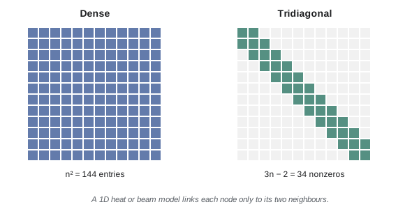
Fortunately, the large matrices of engineering are sparse: each unknown is connected only to its neighbours, so almost all entries are zero. Exploiting sparsity, through banded solvers, sparse direct solvers and iterative methods, is what makes large simulations possible.

Pivoting

Elimination divides by each pivot. If a pivot is zero, the method fails outright; if it is very small, it succeeds but amplifies round-off error enormously.

Partial pivoting chooses, at each step, the row with the largest absolute entry in the pivot column and swaps it into the pivot position. This keeps every multiplier at most 1 in size and makes Gaussian elimination stable in practice. Every serious library does it automatically.

LU factorization

Elimination can be recorded as a factorization \(PA = LU\): U is the upper triangular result, L is lower triangular with 1s on its diagonal and the multipliers below it, and P is the permutation matrix of row swaps. Solving \(A\mathbf{x} = \mathbf{b}\) then takes two quick triangular solves:

The expensive \(\frac{2}{3}n^3\) work is all in the factorization; each solve costs only about \(2n^2\). This is why LU matters in practice. A structural model is analysed for dozens of load combinations (dead, live, snow, wind, earthquake…) with the same stiffness matrix A; it is factored once and each load case is a cheap pair of substitutions.

Conditioning: how accurate can the answer be?

Lesson 1 defined the condition number of a function. For a matrix, the condition number \(\kappa(A) = \|A\|\,\|A^{-1}\|\) bounds how much relative errors in the data can grow in the solution:

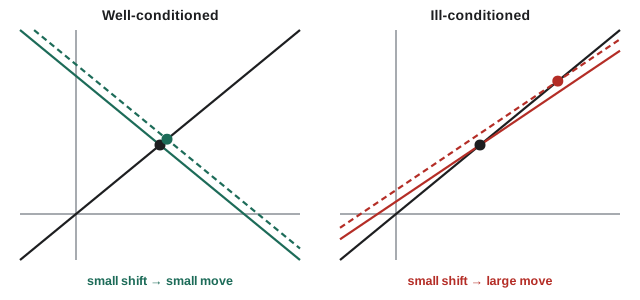
A useful rule of thumb: you can lose up to \(\log_{10}\kappa\) significant digits. With double precision's 16 digits and κ = 10⁴, expect about 12 good digits; with κ = 10¹⁶, possibly none. A nearly singular matrix (rows almost linearly dependent) has a huge condition number.

The Hilbert matrix, with entries \(1/(i + j - 1)\), is the classic ill-conditioned example: κ is about 1.6 × 10⁴ for n = 4, 1.5 × 10¹⁰ for n = 8 and 1.6 × 10¹³ for n = 10. It appears when fitting high-degree polynomials with the normal equations, one reason Lesson 4 warns against that.

Iterative methods for large sparse systems

For very large sparse systems, iterative methods start from a guess and improve it, using only matrix–vector products, which are cheap when most entries are zero. The simplest solve each equation for its diagonal unknown:

• Jacobi: compute every new \(x_i\) from the previous iterate's values.
• Gauss–Seidel: use each new value as soon as it is available, which usually roughly doubles the convergence rate.

Both are guaranteed to converge if A is strictly diagonally dominant (each diagonal entry larger in magnitude than the sum of the others in its row) and Gauss–Seidel also converges for symmetric positive definite matrices, which is what most physical models produce (stiffness, conductance and diffusion matrices).

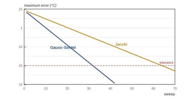
These basic methods slow down badly as grids get finer. Modern practice uses faster relatives: successive over-relaxation (SOR), the conjugate gradient method for symmetric positive definite systems, GMRES for general ones, and preconditioning and multigrid to accelerate them. Together with sparse direct solvers, they are the engines inside finite element, circuit and reservoir simulators.

A special case deserves mention: tridiagonal systems, like the rod, can be solved directly in about 8n operations by the Thomas algorithm, Gaussian elimination that skips all the zeros. Splines (Lesson 4) and implicit ODE and heat-equation solvers use it constantly.

import numpy as np
from scipy.linalg import lu_factor, lu_solve

A = np.array([[ 2.0,  1.0, -1.0],
              [-3.0, -1.0,  2.0],
              [-2.0,  1.0,  2.0]])
b = np.array([8.0, -11.0, -3.0])
print("solve:", np.linalg.solve(A, b))

lu, piv = lu_factor(A)              # factor once...
for rhs in ([8, -11, -3], [1, 0, 0]):
    print("LU solve:", lu_solve((lu, piv), rhs))   # ...solve many times
print(f"cond(A) = {np.linalg.cond(A):.1f}")

B = np.array([[1, 1], [1, 1.0001]])
print(np.linalg.solve(B, [2, 2.0001]), np.linalg.solve(B, [2, 2.0002]))
print(f"cond(B) = {np.linalg.cond(B):.0f}")

Output: solve: [2. 3. −1.]; LU solve: [2. 3. −1.] and [4. −2. 5.]; cond(A) = 44.7; [1. 1.] [0. 2.]; cond(B) = 40002.