Solving ODEs in practice: error control, stiffness and long simulations

Lesson 7 introduced Euler's method and the Runge-Kutta methods with a fixed step, and showed that stiff equations need special treatment. Professional ODE solvers go much further. They choose their own step sizes to meet an accuracy target, switch to implicit methods when an equation is stiff, stop exactly when an event occurs, and, for long simulations of orbits or molecules, preserve the physical structure of the problem. This lesson explains how they do it, so that you can choose a solver, set its tolerances, recognize when a result is untrustworthy, and interpret warnings rather than ignore them. It covers local and global error and how to verify a method's order, adaptive step control with embedded Runge-Kutta pairs, multistep methods, implicit methods and stability regions, stiffness in depth, event detection and symplectic methods for long-time simulation.

Local error, global error and order

Each step of a method commits a local truncation error, the error made in one step starting from exact values. For a method of order p, the local error is proportional to \(h^{p+1}\). Over a fixed interval there are about \(1/h\) steps, and the errors accumulate (and may grow or shrink as the solution evolves), so the global error at the end is proportional to \(h^p\). Halving the step should therefore cut the global error by a factor of \(2^p\): 2 for Euler, 16 for classical RK4.

This gives a practical check on any implementation: solve a problem with a known solution at several step sizes and confirm that the error falls at the expected rate. If it does not, there is a bug, or the solution is not smooth enough for the method's order to apply. When the exact solution is unknown, comparing solutions at h, h/2 and h/4 gives the same information, and Richardson extrapolation (Lesson 7) can combine them into a more accurate answer.

Adaptive step size control

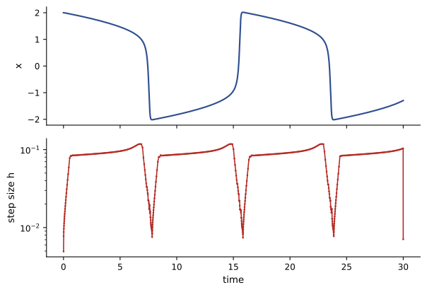
A fixed step wastes effort where the solution is smooth and loses accuracy where it changes quickly. Adaptive solvers estimate the local error at every step and adjust h to keep it near a tolerance. The efficient way to estimate the error is an embedded Runge-Kutta pair: two formulas of different orders (for example 4 and 5) that share the same stage evaluations, so the second costs almost nothing. Their difference estimates the error of the lower-order result. The step is accepted if the estimate is within the tolerance and rejected and retried otherwise, and the next step size is chosen by

where the exponent comes from the error being proportional to \(h^5\) and 0.9 is a safety factor. The Dormand-Prince 5(4) pair, used by scipy's solve_ivp (RK45) and MATLAB's ode45, is the default general-purpose solver in most software.

The tolerance has two parts. The relative tolerance rtol controls the number of correct significant digits; the absolute tolerance atol sets the size below which a component is treated as negligible, which matters when a solution passes through or decays toward zero. Each step aims for an error below \(\text{atol} + \text{rtol} \times |y|\). Defaults (rtol = 10⁻³ in solve_ivp) are loose; for engineering results, tighten them and check that the answer does not change.

Multistep methods

Runge-Kutta methods use several evaluations within each step and then forget them. Multistep methods instead reuse values from previous steps. The second-order Adams-Bashforth method, for example, is

needing only one new evaluation of f per step. Adams methods of high order are very efficient for smooth, non-stiff problems in which f is expensive to evaluate, such as orbit computations. Their drawbacks are that they need a starting procedure (usually a few Runge-Kutta steps) and that changing the step size is more awkward. Implicit multistep methods, the backward differentiation formulas (BDF), are the classic solvers for stiff problems.

Implicit methods and stability regions

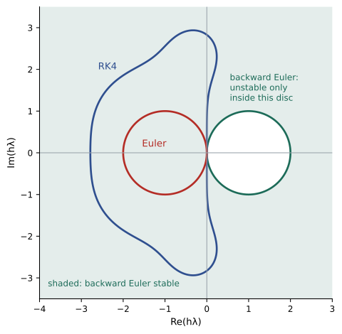
To compare methods on stability, apply them to the test equation \(y' = \lambda y\), whose solution decays when the real part of λ is negative. Euler's method gives \(y_{n+1} = (1 + h\lambda)y_n\), which decays only if \(|1 + h\lambda| \le 1\): \(h\lambda\) must lie in a disc of radius 1 centred at −1, its stability region. The backward (implicit) Euler method evaluates f at the new point:

which decays for every λ with negative real part and every step size. A method with this property is called A-stable. The trapezoidal rule (the Crank-Nicolson method, Lesson 10) is also A-stable and second order. The price of implicitness is that each step requires solving an equation for \(y_{n+1}\), nonlinear in general, by Newton's method (Lesson 2), which needs the Jacobian of f and the solution of a linear system (Lesson 3) at each iteration.

Stiffness

A system is stiff when it contains processes with very different time scales and the fast ones have died away: the solution is smooth, but an explicit method must still take steps small enough to stay stable for the fastest decay rate. Chemical kinetics, circuit simulation (where tiny parasitic capacitances coexist with slow control loops), combustion, heat conduction on fine grids (Lesson 10) and structural dynamics with stiff elements are typically stiff. The eigenvalues of the Jacobian of f measure the time scales; a stiffness ratio of thousands or more between the largest and smallest decay rates is a warning sign.

from scipy.integrate import solve_ivp

# Robertson chemical kinetics: rates differ by nine orders of magnitude (a stiff system)
def robertson(t, y):
    a, b, c = y
    return [-0.04 * a + 1e4 * b * c,
             0.04 * a - 1e4 * b * c - 3e7 * b**2,
             3e7 * b**2]

for method in ["RK45", "Radau", "BDF", "LSODA"]:
    sol = solve_ivp(robertson, [0, 100], [1.0, 0.0, 0.0], method=method, rtol=1e-6, atol=1e-10)
    print(f"{method:6s}: {sol.t.size - 1:6d} steps, {sol.nfev:7d} rate evaluations, y1(100) = {sol.y[0, -1]:.4f}")

RK45  : 104142 steps,  729668 rate evaluations, y1(100) = 0.6172
Radau :     88 steps,     726 rate evaluations, y1(100) = 0.6172
BDF   :    163 steps,     431 rate evaluations, y1(100) = 0.6172
LSODA :    240 steps,     496 rate evaluations, y1(100) = 0.6172

All four solvers agree on the answer, but the explicit RK45 needs over a hundred thousand steps, nearly all forced by stability rather than accuracy, while the implicit methods (Radau, BDF) and LSODA, which switches automatically between Adams and BDF, need a few hundred. A practical rule follows: if an explicit solver takes an unexpectedly large number of steps, or is very slow, on a problem whose solution looks smooth, try an implicit method.

Events

Engineering simulations often need to stop or change when something happens: a projectile hits the ground, a tank empties, a valve opens at a set pressure, a ball bounces. Stepping past the moment and interpolating is inaccurate. Instead, solvers accept an event function g(t, y) and, after each step, check whether g has changed sign; if so, they locate the root precisely using the solver's interpolant and a root-finding method (Lesson 2). In solve_ivp, an event function can be marked terminal (stop the integration) and given a direction (only rising or only falling crossings). A bouncing ball is simulated by stopping at each impact, reversing and scaling the velocity, and restarting.

Long simulations and symplectic methods

Some simulations run for an extremely long time compared with the system's natural period: planetary orbits over millions of years, molecular dynamics over billions of steps, or a satellite constellation over its design life. Even a highly accurate method can then drift: RK4 slowly removes energy from an undamped oscillator, so orbits decay and molecules cool, although the true system conserves energy. Symplectic methods, such as the velocity Verlet (leapfrog) method, preserve the geometric structure of mechanical systems. Their energy error stays bounded, oscillating slightly, instead of drifting, however long the simulation runs.

import numpy as np

# Undamped oscillator: x double-prime = -x (period 2 pi); energy (x^2 + v^2)/2 starts at 0.5
h, periods = 0.5, 1000
n = int(round(periods * 2 * np.pi / h))

def euler(x, v):
    return x + h * v, v - h * x

def rk4(x, v):
    f = lambda x, v: (v, -x)
    k1 = f(x, v)
    k2 = f(x + h / 2 * k1[0], v + h / 2 * k1[1])
    k3 = f(x + h / 2 * k2[0], v + h / 2 * k2[1])
    k4 = f(x + h * k3[0], v + h * k3[1])
    return (x + h / 6 * (k1[0] + 2 * k2[0] + 2 * k3[0] + k4[0]),
            v + h / 6 * (k1[1] + 2 * k2[1] + 2 * k3[1] + k4[1]))

def verlet(x, v):                      # velocity Verlet (leapfrog), a symplectic method
    v_half = v - h / 2 * x
    x_new = x + h * v_half
    return x_new, v_half - h / 2 * x_new

print(f"Step h = {h}; energy starts at 0.5")
n10 = int(round(10 * 2 * np.pi / h))
for name, step in [("Euler", euler), ("RK4", rk4), ("Verlet", verlet)]:
    x, v = 1.0, 0.0
    with np.errstate(over="ignore", invalid="ignore"):
        for i in range(n):
            x, v = step(x, v)
            if i == n10 - 1:
                E10 = 0.5 * (x * x + v * v)
        E = 0.5 * (x * x + v * v)
    E_text = f"{E:.4f}" if np.isfinite(E) else "overflow"
    print(f"{name:7s} after 10 periods {E10:10.4g}   after {periods} periods {E_text}")

Step h = 0.5; energy starts at 0.5
Euler   after 10 periods  8.121e+11   after 1000 periods overflow
RK4     after 10 periods     0.4869   after 1000 periods 0.0356
Verlet  after 10 periods     0.4826   after 1000 periods 0.4728

Euler adds energy at every step and explodes. RK4 is far more accurate over 10 periods, but after 1000 periods it has removed 93% of the energy. Verlet, only second order, keeps the energy within about 6% indefinitely. For long simulations of conservative systems, the qualitative behaviour of the method matters more than its order.

Choosing a solver

A sensible default for an engineering ODE problem is: start with an adaptive explicit method (RK45) and tight tolerances; if it is slow or takes many steps on a smooth solution, switch to an implicit method (Radau or BDF) and supply the Jacobian if it is easy to compute; for long-time conservative mechanics, use a symplectic method; use events for anything that happens at an unknown time. In every case, check the result by tightening the tolerance and confirming that the answer does not change, and compare with an analytical solution of a simplified version.