
MATH-300 · Lesson 10 of 12 · 28 min
Finite difference methods for partial differential equations
The heat, wave and Laplace equations (MATH-201 and MATH-209) govern conduction, vibration, diffusion, seepage, electrostatics and much more, but they can be solved by formula only on simple shapes with simple conditions. Real problems, such as a wall with layers of different materials, a shaft of non-circular section or a soil mass around a foundation, are solved numerically. This lesson develops the finite difference method for PDEs. It starts with the heat equation and three time-stepping schemes (explicit, implicit and Crank-Nicolson), explains why the explicit scheme becomes unstable using von Neumann analysis, and then treats the wave equation and its CFL condition, Laplace's and Poisson's equations in two dimensions with sparse matrices, and the method of lines, which hands the time-stepping to the ODE solvers of Lesson 8. It closes with the practical habits that make PDE results trustworthy.
The heat equation on a grid
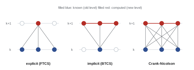
For \(u_t = \alpha u_{xx}\) on \(0 \le x \le L\), place grid points \(x_i = i\,\Delta x\) and time levels \(t_k = k\,\Delta t\), and write \(u_i^k\) for the approximation to \(u(x_i, t_k)\). Replacing \(u_{xx}\) by the centred second difference (Lesson 9) and \(u_t\) by a forward difference gives the explicit, or FTCS (forward time, centred space), scheme:
Each new value is computed directly from three old ones, so a step is very cheap. The scheme is first order in time and second order in space. MATH-201 stated that it is stable only if \(r \le \tfrac{1}{2}\); the next section shows why.
Stability: von Neumann analysis
Errors on the grid can be written as a sum of Fourier modes \(e^{\mathrm{i}\beta x_i}\). Substituting a single mode \(u_i^k = G^k e^{\mathrm{i}\beta i\Delta x}\) into the FTCS scheme gives the amplification factor G, the factor by which that mode is multiplied at each step:
For stability every mode must satisfy \(|G| \le 1\). The worst case is the shortest wave the grid can represent, a sawtooth with \(\sin^2 = 1\), for which \(G = 1 - 4r\). This lies between −1 and 1 only if \(r \le \tfrac{1}{2}\). For larger r the sawtooth mode grows by a factor \(|1 - 4r|\) every step, so round-off errors, always present at the level of 10⁻¹⁶, explode into wild oscillations within a few hundred steps. The restriction is severe: halving \(\Delta x\) to improve accuracy forces \(\Delta t\) to fall by four, so the work rises eightfold.
Worked problem
The time-step limit
A concrete wall 0.20 m thick (α = 1.0 × 10⁻⁶ m²/s) is modelled with 40 intervals. What is the largest stable explicit time step, and how many steps does a 24-hour simulation need?
Show solution
- \(\Delta x = 0.20/40 = 0.005\) m.
- \(\Delta t \le \tfrac{1}{2}\Delta x^2/\alpha = 0.5 \times 2.5 \times 10^{-5}/10^{-6} = 12.5\) s.
- 24 h = 86 400 s needs at least 6912 steps.
Answer: 12.5 s and about 6900 steps, which is trivial for one dimension. On a three-dimensional grid with millimetre spacing the same limit would make an explicit simulation impractical, which is why implicit schemes are used.
Implicit and Crank-Nicolson schemes
Evaluating the spatial difference at the new time level gives the implicit, or BTCS, scheme, and averaging the old and new levels gives the Crank-Nicolson scheme. Both are members of the θ-family:
where \(\delta^2u_i = u_{i-1} - 2u_i + u_{i+1}\). θ = 0 is explicit, θ = 1 implicit and θ = ½ Crank-Nicolson. For θ ≥ ½ the scheme is stable for every r (unconditionally stable), the PDE counterpart of the A-stable ODE methods of Lesson 8. Each step requires solving a tridiagonal system, which costs only O(N), so the large time steps more than repay the extra work per step. Crank-Nicolson is second order in time as well as space; BTCS is only first order in time but damps every mode, which makes it robust for rough initial data, whereas Crank-Nicolson with very large steps lets the sharpest features oscillate briefly before they decay.
import numpy as np
from scipy.linalg import solve_banded

# Wall 0.2 m thick, alpha = 1e-6 m^2/s (concrete), initially 1, both faces suddenly 0
L, alpha, N = 0.2, 1e-6, 40
dx = L / N
x = np.linspace(0, L, N + 1)
t_end = 2 * 3600.0

def exact(t):
    u = np.zeros_like(x)
    for n in range(1, 400, 2):
        u += 4 / (n * np.pi) * np.exp(-alpha * (n * np.pi / L)**2 * t) * np.sin(n * np.pi * x / L)
    return u

def run(theta, r):
    dt = r * dx**2 / alpha
    steps = int(round(t_end / dt))
    dt = t_end / steps
    r = alpha * dt / dx**2
    u = np.ones(N + 1); u[0] = u[-1] = 0.0
    m = N - 1
    ab = np.zeros((3, m))
    ab[0, 1:] = -theta * r; ab[1, :] = 1 + 2 * theta * r; ab[2, :-1] = -theta * r
    for _ in range(steps):
        lap = u[:-2] - 2 * u[1:-1] + u[2:]
        rhs = u[1:-1] + (1 - theta) * r * lap
        if theta == 0:
            u[1:-1] = rhs
        else:
            u[1:-1] = solve_banded((1, 1), ab, rhs)
    return u, steps

ue = exact(t_end)
print(f"Exact mid-plane value after 2 h: {ue[N // 2]:.5f}")
for name, theta in [("explicit (FTCS)", 0.0), ("implicit (BTCS)", 1.0), ("Crank-Nicolson", 0.5)]:
    for r in [0.4, 0.6, 5.0]:
        u, steps = run(theta, r)
        err = np.max(np.abs(u - ue))
        text = f"{err:.2e}" if err < 10 else "unstable"
print(f"{name:16s} r = {r:3.1f}: {steps:5d} steps, max error {text}")Exact mid-plane value after 2 h: 0.21546 explicit (FTCS) r = 0.4: 720 steps, max error 3.86e-04 explicit (FTCS) r = 0.6: 480 steps, max error unstable explicit (FTCS) r = 5.0: 58 steps, max error unstable implicit (BTCS) r = 0.4: 720 steps, max error 5.58e-04 implicit (BTCS) r = 0.6: 480 steps, max error 7.93e-04 implicit (BTCS) r = 5.0: 58 steps, max error 5.90e-03 Crank-Nicolson r = 0.4: 720 steps, max error 8.57e-05 Crank-Nicolson r = 0.6: 480 steps, max error 8.55e-05 Crank-Nicolson r = 5.0: 58 steps, max error 5.61e-05
The explicit scheme is accurate at r = 0.4 and useless at r = 0.6, just past the stability limit. The implicit scheme is stable for any r but loses accuracy at large steps because it is only first order in time. Crank-Nicolson stays accurate even with 58 large steps, which is why it is the default for diffusion problems.
The wave equation and the CFL condition
For \(u_{tt} = c^2u_{xx}\), centred differences in both time and space give an explicit three-level scheme:
Von Neumann analysis shows it is stable if and only if the Courant number C ≤ 1. This Courant-Friedrichs-Lewy (CFL) condition has a physical meaning: in one time step a wave travels \(c\,\Delta t\), and the numerical scheme can only pass information one grid cell per step, so \(c\,\Delta t\) must not exceed \(\Delta x\); the numerical domain of dependence must contain the physical one. The same principle limits time steps in every explicit simulation of waves and fast flows, from acoustics and seismology to crash simulation and weather prediction. At C = 1 the one-dimensional scheme is exact; at smaller C, waves of different lengths travel at slightly wrong speeds, a numerical dispersion that spreads sharp pulses into trailing ripples, so grids need several points per wavelength (ten or more is a common rule).
Laplace and Poisson equations in two dimensions
Steady problems such as \(u_{xx} + u_{yy} = f\) have no time stepping: all grid values are found at once. The five-point stencil replaces the Laplacian at each interior point by
giving one linear equation per interior point. An N × N grid has about N² unknowns, but each equation involves only five of them, so the matrix is sparse: a 1000 × 1000 grid has a million unknowns but only five million non-zero entries. Such systems are solved with sparse direct solvers, which reorder the unknowns to limit fill-in during elimination, or with iterative methods (Gauss-Seidel and over-relaxation from Lesson 3, or the much faster conjugate gradient and multigrid methods for large problems). Storing the matrix densely, with 10¹² entries, would be impossible.
Worked problem
Torsion of a square shaft
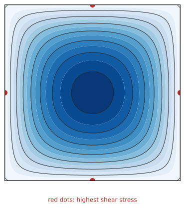
The torsional stiffness of a shaft of any cross-section follows from the Prandtl stress function φ, which satisfies \(\nabla^2\phi = -2\) (in suitable units) inside the section and φ = 0 on its boundary. The torsion constant is \(J = 2\iint\phi\,dA\). For a circle the exact answer is the polar moment of area; for a square of side a, a series solution gives J = 0.1406a⁴. Compute J numerically.
Show solution
- Build the five-point Laplacian on an N × N grid as a sparse matrix (using Kronecker products of the one-dimensional difference matrix).
- Solve for φ with a sparse direct solver and sum to approximate the integral.
Answer: The code reproduces 0.1406a⁴ to four digits on an 80 × 80 grid, with the error falling by four each time h is halved. The same program, with the boundary changed, gives J for an I-beam, a keyed shaft or a hollow section, shapes for which no formula exists.
import numpy as np
import scipy.sparse as sp
from scipy.sparse.linalg import spsolve

# Torsion of a square shaft (side a = 1): Prandtl stress function, laplacian(phi) = -2, phi = 0 on edges
# Torsion constant J = 2 * integral of phi over the section; exact J = 0.14058 a^4
for N in [10, 20, 40, 80]:
    h = 1.0 / N
    n = N - 1                                   # interior points per side
    I = sp.identity(n)
    T = sp.diags([1.0, -2.0, 1.0], [-1, 0, 1], shape=(n, n))
    A = (sp.kron(I, T) + sp.kron(T, I)) / h**2  # five-point Laplacian, sparse
    phi = spsolve(A.tocsc(), -2 * np.ones(n * n))
    J = 2 * phi.sum() * h**2
    print(f"N = {N:3d}: {n * n:5d} unknowns, {A.nnz:6d} non-zeros, J = {J:.5f} a^4")
print("Exact: J = 0.14058 a^4")N = 10: 81 unknowns, 369 non-zeros, J = 0.13612 a^4 N = 20: 361 unknowns, 1729 non-zeros, J = 0.13944 a^4 N = 40: 1521 unknowns, 7449 non-zeros, J = 0.14029 a^4 N = 80: 6241 unknowns, 30889 non-zeros, J = 0.14051 a^4 Exact: J = 0.14058 a^4
The method of lines
An alternative to designing a time-stepping scheme by hand is to discretize only in space, which turns the PDE into a large system of ODEs, \(d\mathbf{u}/dt = A\mathbf{u} + \mathbf{b}\), and pass it to an ODE solver from Lesson 8. This is the method of lines. The solver then controls the time error adaptively. Because the eigenvalues of the discrete diffusion operator range from about \(-\alpha\pi^2/L^2\) to \(-4\alpha/\Delta x^2\), a ratio of roughly \((L/\Delta x)^2\), diffusion problems on fine grids are stiff, so an implicit solver (BDF or Radau, with a sparse Jacobian) should be used. The method of lines is convenient for nonlinear problems, such as conductivity that varies with temperature or reaction terms, and for coupled systems.
Trusting PDE results
Numerical PDE solutions can look convincing while being wrong. Good practice includes: verifying the code on a problem with an exact solution (a manufactured solution can be created by choosing u, computing the source term that makes it exact, and checking the error); refining the grid and confirming that results change at the expected rate; respecting stability limits, or using unconditionally stable schemes; checking conservation (total heat or mass should balance the boundary fluxes); and comparing with simple hand estimates such as a one-term series or a one-dimensional approximation.
Common mistakes
MistakeRunning the explicit heat scheme with r > ½.
InsteadKeep r = αΔt/Δx² ≤ ½, or use an implicit or Crank-Nicolson scheme.
MistakeViolating the CFL condition for waves.
InsteadKeep the Courant number cΔt/Δx at or below 1.
MistakeStoring a two-dimensional Laplacian as a dense matrix.
InsteadUse sparse storage and sparse or iterative solvers.
MistakeUsing an explicit ODE solver in the method of lines for diffusion.
InsteadFine-grid diffusion is stiff; use BDF or Radau.
MistakeReporting a single-grid result.
InsteadRefine the grid and confirm convergence at the expected rate.
Summary and key terms
- The explicit FTCS heat scheme is stable only for r ≤ ½, found by von Neumann analysis.
- Implicit (BTCS) and Crank-Nicolson schemes are unconditionally stable and need a tridiagonal solve each step.
- Crank-Nicolson is second order in time and space; BTCS is robust but first order in time.
- The explicit wave scheme needs the CFL condition cΔt/Δx ≤ 1.
- The five-point stencil turns Laplace and Poisson problems into large sparse linear systems.
- The method of lines discretizes space and uses an ODE solver in time; diffusion gives stiff systems.
- Verify codes with exact or manufactured solutions and grid refinement.
- FTCS scheme
- Forward time, centred space: the explicit scheme for the heat equation.
- Amplification factor
- The factor by which a Fourier mode grows or shrinks each time step.
- Von Neumann analysis
- Stability analysis of a scheme using Fourier modes.
- Unconditionally stable
- Stable for every time step.
- Crank-Nicolson scheme
- A second-order scheme averaging the old and new time levels.
- Courant number
- cΔt/Δx, the distance a wave travels per step in grid cells.
- CFL condition
- The requirement that the Courant number not exceed a limit (1 for the standard wave scheme).
- Five-point stencil
- The standard finite difference approximation of the two-dimensional Laplacian.
- Method of lines
- Discretizing a PDE in space to obtain a system of ODEs in time.
- Manufactured solution
- A chosen exact solution used to verify a PDE code.
Practice problems
Work each problem on paper first, then reveal the answer to check.
For α = 10⁻⁵ m²/s and Δx = 1 mm, find the largest stable explicit Δt.
Show answer
0.5 × 10⁻⁶/10⁻⁵ = 0.05 s.
What happens to the explicit time-step limit if Δx is halved?
Show answer
It falls by a factor of 4.
Find G for the sawtooth mode with r = 0.75 in FTCS.
Show answer
1 − 3 = −2; it doubles and flips sign each step.
Which θ gives the Crank-Nicolson scheme?
Show answer
θ = ½.
What system must be solved each step of an implicit one-dimensional heat scheme?
Show answer
A tridiagonal linear system.
A string has c = 200 m/s and Δx = 0.01 m. What is the largest stable Δt for the explicit wave scheme?
Show answer
5 × 10⁻⁵ s.
How many unknowns and approximate non-zeros does a 200 × 200 interior Poisson grid have?
Show answer
40 000 unknowns; about 200 000 non-zeros.
Write the five-point equation for ∇²u = 0 at a point whose neighbours are 10, 20, 30 and 40.
Show answer
u = (10 + 20 + 30 + 40)/4 = 25.
Why is the method of lines for diffusion stiff?
Show answer
Eigenvalues range from about −απ²/L² to −4α/Δx², a ratio near (L/Δx)².
Describe a manufactured-solution test.
Show answer
Pick u(x, t), compute the source term that makes it satisfy the PDE, solve with that source and compare.
Lesson quiz · 5 questions
Score 60% or more to complete this lesson.
Create a free account to save your progress, take quizzes and earn a certificate.