Trees and spanning trees

Trees are the simplest connected graphs, and they are everywhere in computing: the folders on a disk, the structure of a web page, a family tree, the parse of an arithmetic expression, the decisions in a decision tree, and the routes a network protocol uses to avoid loops. They are also the backbone inside every connected graph. Any connected network contains a tree that reaches every vertex, and choosing the cheapest such tree is one of the oldest and most useful problems in optimization. This lesson proves the basic facts about trees, counts them, and gives two greedy algorithms that find minimum spanning trees.

Definition and the equivalent characterizations

A tree is a connected graph with no cycles. A graph with no cycles, connected or not, is a forest; its components are trees. A vertex of degree 1 in a tree is a leaf.

Lemma. Every tree with at least two vertices has at least two leaves. Proof: take a longest path \(v_0, v_1, \dots, v_k\) in the tree. The end \(v_k\) is adjacent to \(v_{k-1}\). If it had another neighbour \(w\), either \(w\) is on the path, which would create a cycle, or \(w\) is not, which would give a longer path. Neither is possible, so \(v_k\) is a leaf, and by the same argument so is \(v_0\).

Theorem. A tree with \(n\) vertices has exactly \(n - 1\) edges. Proof by induction on \(n\). A tree with one vertex has no edges. For \(n \ge 2\), remove a leaf and its single edge. What remains is still connected, since no path between two other vertices passed through a leaf, and still has no cycles, so it is a tree with \(n - 1\) vertices, which by the induction hypothesis has \(n - 2\) edges. Putting the leaf back gives \(n - 1\) edges.

Theorem. For a graph \(G\) with \(n\) vertices, the following are equivalent:

• \(G\) is a tree, that is, connected with no cycles.

• \(G\) is connected and has \(n - 1\) edges.

• \(G\) has no cycles and has \(n - 1\) edges.

• There is exactly one path between every pair of vertices.

• \(G\) is connected, and removing any edge disconnects it; trees are the minimally connected graphs.

• \(G\) has no cycles, and adding any edge creates exactly one cycle; trees are the maximally acyclic graphs.

The proofs all use the same few ideas: the count from Lesson 8 that each edge can reduce the number of components by at most one, and the fact that a second path between two vertices would create a cycle. For example, if \(G\) has no cycles and \(n - 1\) edges, add the edges one at a time to \(n\) isolated vertices. No edge ever closes a cycle, so each one joins two components, and after \(n - 1\) edges there is a single component. The equivalences make it easy to check a tree in practice: count the edges and test connectivity.

Rooted trees

Choosing one vertex as the root turns a tree into a hierarchy. Every other vertex then has a unique parent, the next vertex on its path toward the root, and its children are the neighbours further away. The depth of a vertex is its distance from the root, and the height of the tree is the largest depth. A binary tree is a rooted tree in which each vertex has at most two children, labelled left and right.

Counting gives the basic size bounds. A binary tree of height \(h\) has at most \(1 + 2 + 4 + \dots + 2^h = 2^{h+1} - 1\) vertices, so a binary tree with \(n\) vertices has height at least \(\log_2(n + 1) - 1\). This is why balanced search trees, which keep their height close to \(\log_2 n\), can find any of a million keys in about 20 comparisons. It also gives a lower bound on sorting: a comparison sort is a binary decision tree whose leaves are the \(n!\) possible orderings, so its height, the worst-case number of comparisons, is at least \(\log_2 n!\), which is about \(n \log_2 n\). CMPUT-204 develops these ideas.

In a full binary tree, where every vertex has 0 or 2 children, the number of leaves is one more than the number of internal vertices. Count edges two ways: each of the \(i\) internal vertices has two children, so there are \(2i\) edges; but a tree with \(i + \ell\) vertices has \(i + \ell - 1\) edges. Setting them equal gives \(\ell = i + 1\). This is why a knockout tournament with 64 players has exactly 63 matches: every match eliminates one player.

Counting labelled trees: Cayley's formula

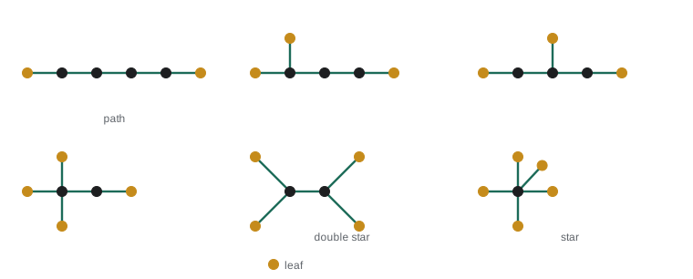
How many different trees can be built on the vertex set \(\{1, 2, \dots, n\}\)? For \(n = 3\) there are 3, since a tree on three vertices is a path and the middle vertex can be any of the three. For \(n = 4\) there are 16: 12 paths and 4 stars. The general answer is remarkably simple.

Theorem (Cayley's formula). The number of labelled trees on \(n\) vertices is \(n^{n-2}\).

The formula is named after Arthur Cayley, who wrote about it in 1889, although Carl Borchardt had proved it in 1860. A beautiful proof was given by Heinz Prüfer in 1918, who found a bijection between labelled trees and sequences of length \(n - 2\) with entries from \(\{1, \dots, n\}\). There are \(n^{n-2}\) such sequences by the product rule, so the bijection proves the formula.

The Prüfer code of a tree is built as follows. Repeatedly remove the leaf with the smallest label, and write down the label of its neighbour, until only two vertices remain. The code records \(n - 2\) labels. To decode, note that a vertex appears in the code exactly (degree minus 1) times; leaves never appear. Given the code, the first leaf removed was the smallest label not in the code, and it was attached to the first entry of the code; remove that leaf from consideration and the first code entry, and repeat. At the end, join the two remaining vertices. Each step is forced, so every sequence comes from exactly one tree.

Spanning trees

A spanning tree of a connected graph \(G\) is a subgraph that is a tree and includes every vertex. Every connected graph has one: while the graph has a cycle, remove an edge of that cycle, which keeps the graph connected because the rest of the cycle is a detour; when no cycles remain we have a spanning tree. Alternatively, the edges used by a breadth-first or depth-first search form a spanning tree. Cayley's formula counts the spanning trees of \(K_n\); Kirchhoff's matrix-tree theorem of 1847, discovered while he was studying electrical circuits, counts the spanning trees of any graph using a determinant.

Spanning trees solve the problem of loops in networks. Ethernet switches connected in a mesh for redundancy would forward broadcast messages around the cycles forever. The spanning tree protocol, designed by Radia Perlman in 1985, has the switches agree on a spanning tree and disable the other links, keeping them in reserve in case a tree link fails.

Minimum spanning trees

Now give each edge a weight, such as the cost of laying a cable. A minimum spanning tree (MST) is a spanning tree whose total weight is as small as possible. Two greedy algorithms find one, and the reason both work is a single fact about cuts.

Cut property. Split the vertices into two nonempty sets \(S\) and \(V \setminus S\). If \(e\) is an edge of smallest weight among those crossing between the two sets, then some minimum spanning tree contains \(e\).

Proof. Let \(T\) be a minimum spanning tree. If \(T\) contains \(e = uv\), we are done. Otherwise, adding \(e\) to \(T\) creates a cycle. This cycle goes from \(u\) on one side to \(v\) on the other and back, so it crosses between the sets at least one more time, along some edge \(f\) of \(T\). Replace \(f\) by \(e\). The result is still connected with \(n - 1\) edges, so it is a spanning tree, and its weight is \(w(T) - w(f) + w(e) \le w(T)\) because \(e\) was the lightest crossing edge. So it is also a minimum spanning tree, and it contains \(e\).

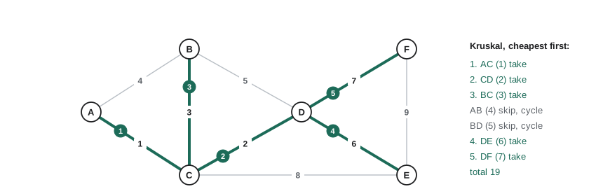
Kruskal's algorithm (Joseph Kruskal, 1956): sort the edges from lightest to heaviest and go through them in order, adding an edge whenever it does not create a cycle with the edges already chosen. Each added edge joins two components of the forest built so far, and it is the lightest edge crossing between the component on one side and the rest of the graph, so the cut property says it is safe. Detecting whether an edge would create a cycle means checking whether its ends are already in the same component, which the union-find data structure does almost instantly.

Prim's algorithm (Vojtěch Jarník, 1930; rediscovered by Robert Prim in 1957 and Edsger Dijkstra in 1959): grow a single tree from a starting vertex, at each step adding the lightest edge from the tree to a vertex not yet in it. That edge is the lightest crossing the cut between the tree and the rest, so again the cut property justifies it. The first MST algorithm of all was published by Otakar Borůvka in 1926, to plan an efficient electrical network for the region of Moravia.

import heapq

def kruskal(n, edges):
    parent = list(range(n))
    def find(x):
        while parent[x] != x:
            parent[x] = parent[parent[x]]   # path halving
            x = parent[x]
        return x
    tree, total = [], 0
    for w, u, v in sorted(edges):
        ru, rv = find(u), find(v)
        if ru != rv:              # different components: no cycle
            parent[ru] = rv
            tree.append((u, v, w)); total += w
    return tree, total

def prim(n, edges, start=0):
    adj = [[] for _ in range(n)]
    for w, u, v in edges:
        adj[u].append((w, v)); adj[v].append((w, u))
    in_tree, total, heap = {start}, 0, [(w, start, v) for w, v in adj[start]]
    heapq.heapify(heap)
    order = []
    while heap and len(in_tree) < n:
        w, u, v = heapq.heappop(heap)
        if v in in_tree:
            continue
        in_tree.add(v); total += w; order.append((u, v, w))
        for w2, x in adj[v]:
            if x not in in_tree:
                heapq.heappush(heap, (w2, v, x))
    return order, total

names = "ABCDEF"
E = [(4, 0, 1), (1, 0, 2), (3, 1, 2), (5, 1, 3), (2, 2, 3),
     (8, 2, 4), (6, 3, 4), (7, 3, 5), (9, 4, 5)]
t, c = kruskal(6, E)
print("Kruskal:", [names[u] + names[v] + "=" + str(w) for u, v, w in t], "total", c)
t, c = prim(6, E)
print("Prim:   ", [names[u] + names[v] + "=" + str(w) for u, v, w in t], "total", c)

def prufer(n, edges):
    nbrs = {v: set() for v in range(1, n + 1)}
    for u, v in edges:
        nbrs[u].add(v); nbrs[v].add(u)
    code = []
    for _ in range(n - 2):
        leaf = min(v for v in nbrs if len(nbrs[v]) == 1)
        (nb,) = nbrs[leaf]
        code.append(nb); nbrs[nb].discard(leaf); del nbrs[leaf]
    return code

print("Prufer code:", prufer(6, [(1, 2), (2, 3), (3, 4), (3, 5), (5, 6)]))

from itertools import combinations
def count_trees(n):
    vs = range(n)
    count = 0
    for es in combinations(list(combinations(vs, 2)), n - 1):
        parent = list(vs)
        def find(x):
            while parent[x] != x:
                x = parent[x]
            return x
        ok = True
        for u, v in es:
            a, b = find(u), find(v)
            if a == b:
                ok = False; break
            parent[a] = b
        count += ok
    return count

for n in range(2, 7):
    print(n, "vertices:", count_trees(n), "trees on numbered vertices; n^(n-2) =", n ** (n - 2))

Kruskal: ['AC=1', 'CD=2', 'BC=3', 'DE=6', 'DF=7'] total 19
Prim:    ['AC=1', 'CD=2', 'CB=3', 'DE=6', 'DF=7'] total 19
Prufer code: [2, 3, 3, 5]
2 vertices: 1 trees on numbered vertices; n^(n-2) = 1
3 vertices: 3 trees on numbered vertices; n^(n-2) = 3
4 vertices: 16 trees on numbered vertices; n^(n-2) = 16
5 vertices: 125 trees on numbered vertices; n^(n-2) = 125
6 vertices: 1296 trees on numbered vertices; n^(n-2) = 1296

Both algorithms find a tree of cost 19 for the six offices; here they even add the edges in the same order, though on other graphs Prim’s order follows the growing tree rather than the weights. When all edge weights are different, the minimum spanning tree is unique, so any correct algorithm returns the same tree. A warning about greed: it works for spanning trees because of the cut property, but the similar-sounding problem of the cheapest Hamilton cycle from Lesson 8 is not solved by any known greedy rule.