Partial differential equations and Fourier series

Everything so far has involved ordinary differential equations, where the unknown depends on a single variable, usually time. Many engineering quantities depend on position as well: the temperature through a wall as it heats up, the displacement of a vibrating string or beam, the stress in a dam, the pressure in an aquifer, the voltage along a transmission line. Their governing laws are partial differential equations (PDEs), which relate rates of change in time and space. This lesson introduces the three classic PDEs of engineering, the heat, wave and Laplace equations, and solves them on simple shapes by separation of variables. The method reduces each PDE to the ordinary differential equations and eigenvalue problems of earlier lessons, and assembles the solution from the eigenfunctions of Lesson 6 using Fourier series. It ends with a finite-difference solution, the starting point of the numerical methods used for real geometries.

Three classic equations

The heat (diffusion) equation describes conduction of heat, diffusion of a chemical and consolidation of soil. For temperature \(u(x, t)\) in a rod or slab, an energy balance on a thin slice combined with Fourier's law of conduction gives:

The thermal diffusivity \(\alpha\) (m²/s) measures how fast temperature changes spread. The equation says that a point warms when it is colder than the average of its neighbours, which is what a positive curvature \(u_{xx}\) means.

The wave equation describes a taut string, sound in a pipe, axial vibration of a bar and voltage on a lossless transmission line. For a string with tension T and mass per length \(\mu\), Newton's second law on a short element gives:

Laplace's equation describes steady states: the final temperature in a plate, groundwater seepage, electrostatic potential and ideal fluid flow:

These are the prototypes of the three types of second-order PDE: parabolic (heat: disturbances diffuse and smooth out), hyperbolic (wave: disturbances travel at finite speed) and elliptic (Laplace: every point depends on the whole boundary). Each needs its own kind of conditions: the heat equation needs an initial temperature and boundary conditions; the wave equation needs an initial shape and velocity; Laplace's equation needs conditions all around the boundary.

Fourier sine series

Lesson 6 showed that the eigenfunctions \(\sin(n\pi x/L)\) of \(X'' + \lambda X = 0\) with fixed ends are orthogonal on \(0 \le x \le L\). Almost any function on that interval can be written as a sum of them, a Fourier sine series:

The coefficient formula comes from orthogonality: multiply both sides by \(\sin(m\pi x/L)\) and integrate; every term except \(n = m\) vanishes, and the surviving integral is \(L/2\). It is the same idea as finding the components of a vector by taking dot products with perpendicular unit vectors (MATH-125).

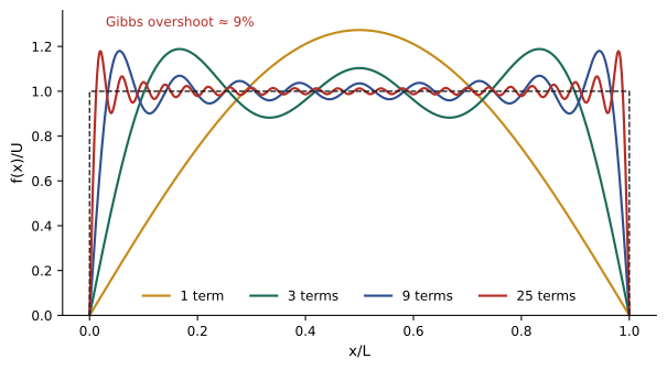
Near a jump, the partial sums overshoot by about 9% of the jump however many terms are taken; this is the Gibbs phenomenon. For periodic signals on \(-L < x < L\), the full Fourier series uses both sines and cosines, \(f = a_0 + \sum (a_n\cos\tfrac{n\pi x}{L} + b_n\sin\tfrac{n\pi x}{L})\), and is the basis of harmonic analysis in power systems and of signal processing, where a square wave from a switching converter is a sum of odd harmonics in exactly this way.

The heat equation by separation of variables

Consider a slab of thickness L, initially at temperature \(f(x)\), whose faces are suddenly held at 0 (measuring temperature relative to the surroundings). Try a solution that is a product of a function of x and a function of t: \(u = X(x)\,G(t)\). Substituting into \(u_t = \alpha u_{xx}\) and dividing by \(\alpha XG\):

The left side depends only on t and the middle only on x, so both must equal the same constant, written \(-\lambda\). This separates the PDE into two ODEs. The space equation \(X'' + \lambda X = 0\) with \(X(0) = X(L) = 0\) is the eigenvalue problem of Lesson 6, with \(\lambda_n = (n\pi/L)^2\) and \(X_n = \sin(n\pi x/L)\). The time equation \(G' = -\alpha\lambda_nG\) gives exponential decay. Adding all the product solutions (superposition) and matching the initial condition with a Fourier series:

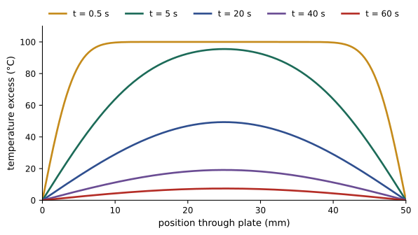
Each mode decays at its own rate, and the rate grows as \(n^2\). The fine-scale wiggles disappear almost at once, and after a short time only the first mode matters: a single sine arch decaying with time constant \(L^2/(\alpha\pi^2)\).

The wave equation: a plucked string

For a string fixed at \(x = 0\) and \(x = L\), separation of variables gives the same space eigenfunctions, but the time equation is now \(G'' = -c^2\lambda_nG\), which oscillates. The solution is a sum of the normal modes found in Lesson 6:

The coefficients \(A_n\) are the sine series coefficients of the initial shape and the \(B_n\) come from the initial velocity. Unlike the heat equation, no mode decays (without damping), so the mix of modes set up at the start persists and determines the sound or vibration.

D'Alembert found another form of the solution, \(u = F(x - ct) + G(x + ct)\): two shapes travelling in opposite directions at speed c, reflecting at the ends. The modal sum and the travelling waves are two descriptions of the same motion.

Laplace's equation in a rectangle

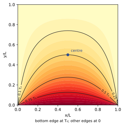
For the steady temperature in a rectangular plate \(0 < x < L\), \(0 < y < H\), with the bottom edge held at \(T_0\) and the other three edges at 0, separation \(u = X(x)Y(y)\) gives the sine eigenfunctions in x again, while the y equation \(Y'' = (n\pi/L)^2Y\) has hyperbolic solutions. Choosing the combination that vanishes at the top edge:

Numerical solution by finite differences

Separation of variables needs simple shapes and linear equations. For everything else, engineers discretize. The finite-difference method replaces derivatives with differences on a grid: for the heat equation, with spacing \(\Delta x\) and time step \(\Delta t\),

This explicit scheme is simple but is stable only if \(r \le \tfrac{1}{2}\); larger time steps make errors grow explosively. The code compares it with the series for the quenched plate.

import numpy as np

# Steel plate 50 mm thick, initially 100 C above the bath, faces at bath temperature
alpha, L, U = 1.2e-5, 0.05, 100.0

def series(x, t, terms):
    u = 0.0
    for n in range(1, 2 * terms, 2):
        u += 4 * U / (n * np.pi) * np.exp(-alpha * (n * np.pi / L)**2 * t) * np.sin(n * np.pi * x / L)
    return u

def finite_difference(t_end, nx=51, r=0.4):
    dx = L / (nx - 1)
    dt = r * dx**2 / alpha
    steps = int(round(t_end / dt))
    dt = t_end / steps
    r = alpha * dt / dx**2
    u = np.full(nx, U)
    u[0] = u[-1] = 0.0
    for _ in range(steps):
        u[1:-1] = u[1:-1] + r * (u[2:] - 2 * u[1:-1] + u[:-2])
    return u[nx // 2], r

for t in [5, 20, 60]:
    one = series(L / 2, t, 1)
    many = series(L / 2, t, 200)
    fd, r = finite_difference(t)
    print(f"t = {t:2d} s: series 1 term {one:6.2f}, 200 terms {many:6.2f}, finite difference {fd:6.2f} (r = {r:.3f})")

fd_bad, r_bad = finite_difference(60, r=0.55)
print(f"Explicit scheme with r = {r_bad:.3f}: mid-plane value {fd_bad:.3g} (unstable)")

t =  5 s: series 1 term 100.47, 200 terms  95.50, finite difference  95.51 (r = 0.400)
t = 20 s: series 1 term  49.37, 200 terms  49.36, finite difference  49.32 (r = 0.400)
t = 60 s: series 1 term   7.42, 200 terms   7.42, finite difference   7.41 (r = 0.400)
Explicit scheme with r = 0.550: mid-plane value -6.18e+101 (unstable)

The series converges quickly once t is not tiny, and the finite-difference result agrees to a fraction of a degree. With r just above ½, the same scheme produces nonsense. Commercial finite element and finite volume programs solve the same equations on complex three-dimensional geometries, and they are checked against exact solutions such as these.