
MATH-101 · Lesson 5 of 12 · 40 min
Separable and linear first-order differential equations
Calculus I introduced differential equations through the simplest cases: \(y' = f(x)\), solved by antidifferentiation, and \(y' = ky\), whose solutions are exponentials, together with Newton's law of cooling and Euler's method. With the integration techniques of Lessons 1 and 2, a much wider class of equations can now be solved exactly. This lesson covers the two most important families of first-order equations. Separable equations, in which the variables can be moved to opposite sides, describe tank draining, population growth with limits, chemical reactions and falling objects with air resistance. Linear equations, solved with an integrating factor, describe mixing tanks, electrical circuits with time-varying sources and the heating of objects whose surroundings change. Together they cover a large share of the first-order models used in engineering, and they prepare you for the systematic treatment in MATH-201.
Separable equations
A first-order differential equation is separable if it can be written as:
that is, the right side is a product of a function of \(x\) alone and a function of \(y\) alone. To solve it, separate the variables by moving everything involving \(y\) to one side and everything involving \(x\) to the other, then integrate both sides:
The result is an equation relating \(x\) and \(y\), with one constant of integration, which an initial condition then fixes. Solve for \(y\) explicitly where possible. The method is justified by the chain rule: if \(H\) is an antiderivative of \(1/h\), then \(\frac{d}{dx}H(y) = \frac{1}{h(y)}\frac{dy}{dx} = g(x)\).
Two cautions apply. Dividing by \(h(y)\) loses any constant solutions where \(h(y) = 0\), which should be checked separately because they are often physically important (an empty tank, a population of zero, an equilibrium). And the solution may exist only on a limited interval, for example until a tank empties.
Worked problem
A first separable equation
Solve \(\dfrac{dy}{dx} = \dfrac{x}{y}\) with \(y(0) = 3\).
Show solution
- Separate: \(y\,dy = x\,dx\).
- Integrate: \(\tfrac{1}{2}y^2 = \tfrac{1}{2}x^2 + C\), so \(y^2 = x^2 + 2C\).
- Initial condition: \(9 = 0 + 2C\). So \(y^2 = x^2 + 9\), and since \(y(0) > 0\), \(y = \sqrt{x^2 + 9}\).
Answer: y = √(x² + 9), the upper branch of a hyperbola.
Draining a tank: Torricelli's law
Water flowing out of a small hole at the bottom of an open tank leaves with a speed of about \(\sqrt{2gh}\), where \(h\) is the depth of water above the hole, a result known as Torricelli's law (it follows from energy conservation, as fluid mechanics courses show). If the hole has area \(a\) and a discharge coefficient \(C_d\) (about 0.6 for a sharp-edged orifice, accounting for the contraction of the jet), the volume flow rate out is \(C_d a\sqrt{2gh}\). For a tank with constant cross-sectional area \(A\), conservation of volume gives:
This equation is separable: \(h^{-1/2}\,dh = -k\,dt\) with \(k = C_d a\sqrt{2g}/A\). Integrating gives \(2\sqrt{h} = -kt + C\), so \(\sqrt{h}\) falls linearly with time:
Worked problem
Time to drain a tank
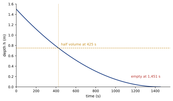
A cylindrical water tank 2.0 m in diameter holds water 1.5 m deep. It drains through a 50 mm diameter sharp-edged hole in the bottom with \(C_d = 0.61\). How long does it take to empty, and how long to drain the first half of its volume?
Show solution
- Areas: \(A = \pi \times 1.0^2 = 3.142\) m²; \(a = \pi \times 0.025^2 = 1.963 \times 10^{-3}\) m².
- \(k = 0.61 \times 1.963 \times 10^{-3} \times \sqrt{19.62} / 3.142 = 1.688 \times 10^{-3}\) m^(1/2)/s.
- Empty: \(t = 2\sqrt{1.5}/k = 2.449/1.688 \times 10^{-3} = 1{,}451\) s, about 24 minutes.
- Half volume (depth 0.75 m): \(t = 2(\sqrt{1.5} - \sqrt{0.75})/k = 2(1.2247 - 0.8660)/1.688 \times 10^{-3} = 425\) s.
Answer: About 24 minutes to empty, but only about 7 minutes for the first half: the flow slows as the depth falls, so the second half takes more than twice as long as the first. Tanks with varying cross-section (cones, spheres, horizontal cylinders) give separable equations with A(h) on the left, solved the same way.
Logistic growth
Exponential growth cannot continue forever: populations run out of food and space, an epidemic runs out of susceptible people, and the adoption of a new technology saturates the market. The logistic equation models growth that slows as it approaches a limit \(K\), the carrying capacity:
For small \(P\), the growth is nearly exponential at rate \(r\); as \(P\) approaches \(K\), growth stops. Separating and using partial fractions (Lesson 1), \(\dfrac{K}{P(K - P)} = \dfrac{1}{P} + \dfrac{1}{K - P}\), gives \(\ln\left|\dfrac{P}{K - P}\right| = rt + C\), and solving for \(P\):
The graph is an S-shaped curve whose growth is fastest at \(P = K/2\), the inflection point. Logistic curves are used to model the market share of new technologies, such as electric vehicles, the growth of microbial cultures in bioreactors, and the spread of infections in their early stages.
Worked problem
Adoption of a technology
In a region, 2 percent of new cars sold are electric in year 0, and adoption follows a logistic curve with \(r = 0.45\) per year toward \(K = 90\) percent of sales. When will electric vehicles reach half of new sales?
Show solution
- \(A = (90 - 2)/2 = 44\), so \(P(t) = \dfrac{90}{1 + 44e^{-0.45t}}\).
- Set \(P = 50\): \(1 + 44e^{-0.45t} = 1.8\), so \(e^{-0.45t} = 0.01818\) and \(t = \ln(55)/0.45 = 8.9\) years.
Answer: About 9 years. The model is only as good as its parameters, and policy, prices and supply constraints can shift both r and K; forecasters fit logistic curves to early data and update them as data accumulate.
Other separable models
Worked problem
A second-order reaction
In a reaction \(2A \to\) products, the concentration falls as \(\dfrac{dc}{dt} = -kc^2\). Find \(c(t)\) and the half-life for \(c_0 = 0.5\) mol/L and \(k = 0.04\) L/(mol·s).
Show solution
- Separate: \(c^{-2}\,dc = -k\,dt\); integrate: \(-1/c = -kt + C\).
- With \(c(0) = c_0\): \(\dfrac{1}{c} = \dfrac{1}{c_0} + kt\).
- Half-life: \(\dfrac{2}{c_0} = \dfrac{1}{c_0} + kt_{1/2}\), so \(t_{1/2} = \dfrac{1}{kc_0} = \dfrac{1}{0.04 \times 0.5} = 50\) s.
Answer: c(t) = 1/(2 + 0.04t) mol/L and a half-life of 50 s. Unlike first-order decay, the half-life of a second-order reaction depends on the starting concentration, a property chemists use to identify reaction order from data (CHEM-103).
Worked problem
Falling with quadratic drag
For fast objects, air drag grows with the square of speed: \(m\dfrac{dv}{dt} = mg - cv^2\). Find the terminal velocity and \(v(t)\) for an object starting from rest.
Show solution
- Terminal velocity (where \(dv/dt = 0\)): \(v_t = \sqrt{mg/c}\). The equation becomes \(\dfrac{dv}{dt} = g\left(1 - \dfrac{v^2}{v_t^2}\right)\).
- Separate and use partial fractions: \(\displaystyle\int \frac{v_t^2\,dv}{v_t^2 - v^2} = \frac{v_t}{2}\ln\frac{v_t + v}{v_t - v} = gt\).
- Solve for \(v\): \(v(t) = v_t \tanh\left(\dfrac{gt}{v_t}\right)\).
Answer: v(t) = vₜ tanh(gt/vₜ), approaching vₜ = √(mg/c). A skydiver with vₜ = 55 m/s reaches 90 percent of terminal velocity after about 8 seconds. The hyperbolic tangent appears naturally from the logarithm, as Lesson 2's inverse hyperbolic functions suggest.
Linear first-order equations
A first-order equation is linear if it can be written in the standard form:
where \(P\) and \(Q\) depend only on \(x\). Such equations are generally not separable when \(Q \ne 0\), but they can always be solved by multiplying through by an integrating factor:
The integrating factor is chosen so that the left side becomes the derivative of a product: \(\mu y' + \mu P y = (\mu y)'\), because \(\mu' = \mu P\). The equation becomes \((\mu y)' = \mu Q\), and integrating gives:
The steps are: write the equation in standard form, compute \(\mu\) (no constant is needed in its exponent), multiply through, recognize the left side as \((\mu y)'\), integrate, and divide by \(\mu\).
Worked problem
An integrating factor
Solve \(y' + 2y = 6e^{x}\) with \(y(0) = 5\).
Show solution
- \(P = 2\), so \(\mu = e^{2x}\). Multiply: \((e^{2x}y)' = 6e^{3x}\).
- Integrate: \(e^{2x}y = 2e^{3x} + C\), so \(y = 2e^{x} + Ce^{-2x}\).
- Initial condition: \(5 = 2 + C\), so \(C = 3\).
Answer: y = 2eˣ + 3e^(−2x). The solution has two parts: a particular response 2eˣ that follows the forcing, and a transient 3e^(−2x) that decays, a structure that recurs throughout the study of linear systems.
Mixing problems
Mixing problems track the amount of a substance in a well-stirred tank as liquid flows in and out. The rate of change of the amount equals the rate in minus the rate out, and the rate out is the outflow rate times the current concentration. Such models describe chemical reactors, water treatment basins, the dilution of pollutants in a lake and the clearance of a drug from the blood.
Worked problem
Salt in a tank
A 1,000 L tank initially contains pure water. Brine with 0.2 kg of salt per litre flows in at 10 L/min, and the well-mixed solution flows out at 10 L/min. Find the amount of salt \(S(t)\) and the time to reach 90 percent of its final value.
Show solution
- Rate in: \(0.2 \times 10 = 2\) kg/min. Rate out: \(10 \times S/1000 = 0.01S\) kg/min.
- Equation: \(S' + 0.01S = 2\), linear with \(\mu = e^{0.01t}\).
- \((e^{0.01t}S)' = 2e^{0.01t}\), so \(e^{0.01t}S = 200e^{0.01t} + C\); with \(S(0) = 0\), \(C = -200\).
- \(S(t) = 200(1 - e^{-0.01t})\) kg. 90 percent: \(e^{-0.01t} = 0.1\), \(t = 230\) min.
Answer: The salt approaches 200 kg (0.2 kg/L throughout the tank) with a time constant of 100 minutes, the tank volume divided by the flow rate, reaching 90 percent after about 3.8 hours. Engineers call this time constant the hydraulic residence time.
If the inflow and outflow rates differ, the volume changes with time, \(V(t) = V_0 + (q_{in} - q_{out})t\), and the coefficient \(P(t) = q_{out}/V(t)\) is no longer constant, but the integrating factor method still applies.
Circuits with time-varying sources
A resistor and inductor in series, driven by a source voltage \(v(t)\), obey Kirchhoff's voltage law, \(L\dfrac{di}{dt} + Ri = v(t)\), a linear first-order equation with time constant \(\tau = L/R\). For a constant source the current rises exponentially to \(V/R\); for a sinusoidal source, the integrating factor method gives a transient that dies away and a steady sinusoidal current that lags the voltage.
Worked problem
RL circuit with a sinusoidal source
Find the steady-state current for \(L\,i' + Ri = V_m\sin\omega t\) with \(R = 10\) Ω, \(L = 0.05\) H, \(V_m = 170\) V and \(\omega = 377\) rad/s.
Show solution
- Using \(\mu = e^{Rt/L}\) and integrating \(e^{at}\sin\omega t\) by parts twice (Lesson 1), the steady-state part of the solution is \(i_{ss} = \dfrac{V_m}{R^2 + \omega^2L^2}\left(R\sin\omega t - \omega L\cos\omega t\right)\).
- This equals \(\dfrac{V_m}{\sqrt{R^2 + (\omega L)^2}}\sin(\omega t - \phi)\) with \(\phi = \arctan(\omega L/R)\).
- Numbers: \(\omega L = 18.85\) Ω; \(\sqrt{100 + 355.3} = 21.34\) Ω; amplitude \(170/21.34 = 7.97\) A; \(\phi = \arctan(1.885) = 62.1°\).
Answer: A steady current of amplitude 7.97 A lagging the voltage by 62°. The quantity √(R² + ω²L²) is the impedance of the circuit; the phasor methods of the ELE circuit courses obtain the same result with complex numbers (Lesson 9) instead of integration by parts.
Choosing a method
For a first-order equation \(y' = F(x, y)\), check in order: Is it of the form \(y' = f(x)\)? Integrate directly. Can \(F\) be factored as \(g(x)h(y)\)? Separate. Can it be written as \(y' + P(x)y = Q(x)\)? Use an integrating factor. Some equations are both separable and linear (\(y' = ky\), the cooling law); either method works. Equations that are neither are solved by special substitutions, by qualitative methods such as slope fields, or numerically with Euler's method and its more accurate successors, which MATH-300 covers.
Common mistakes
MistakeDividing by h(y) and forgetting constant solutions.
InsteadCheck where h(y) = 0; these equilibria are often physically important.
MistakeAdding the constant of integration only after solving for y.
InsteadAdd it when integrating, then solve; in exponentials it becomes a multiplicative constant.
MistakeApplying the integrating factor before writing the equation in standard form.
InsteadDivide by the coefficient of y′ first so the equation reads y′ + P y = Q.
MistakeForgetting to multiply Q(x) by the integrating factor.
InsteadMultiply every term: (μy)′ = μQ.
MistakeAssuming a draining tank empties at a constant rate.
InsteadOutflow depends on √h, so the flow slows as the tank empties.
Summary and key terms
- Separable equations y′ = g(x)h(y) are solved by integrating dy/h(y) = g(x) dx.
- Check constant solutions lost by dividing by h(y), and note intervals of validity.
- Torricelli draining gives √h falling linearly; the first half drains much faster than the second.
- The logistic equation gives S-shaped growth P = K/(1 + Ae^(−rt)) with fastest growth at K/2.
- Quadratic drag gives v = vₜ tanh(gt/vₜ); second-order reactions have concentration-dependent half-lives.
- Linear equations y′ + Py = Q are solved with the integrating factor μ = e^(∫P dx).
- Mixing tanks and RL circuits are linear: transients decay with a time constant, leaving the forced response.
- Separable equation
- A differential equation of the form y′ = g(x)h(y).
- Constant (equilibrium) solution
- A solution y = constant where h(y) = 0.
- Torricelli's law
- Outflow speed from an orifice is about √(2gh).
- Discharge coefficient
- A factor reducing ideal orifice flow to account for jet contraction.
- Logistic equation
- dP/dt = rP(1 − P/K), modelling growth toward a limit.
- Carrying capacity
- The limiting value K in logistic growth.
- Linear first-order equation
- An equation y′ + P(x)y = Q(x).
- Integrating factor
- The multiplier e^(∫P dx) that makes the left side an exact derivative.
- Residence time
- Tank volume divided by flow rate, the time constant of a mixing tank.
- Impedance
- The ratio of voltage amplitude to current amplitude in an AC circuit.
Practice problems
Work each problem on paper first, then reveal the answer to check.
Solve \(y' = 3x^2 y\) with \(y(0) = 2\).
Show answer
y = 2e^(x³).
Solve \(y' = y^2\) with \(y(0) = 1\). Where does the solution exist?
Show answer
y = 1/(1 − x), valid for x < 1.
What constant solutions does \(y' = y(1 - y)\) have?
Show answer
y = 0 and y = 1.
A tank drains from 4 m depth in 20 minutes. How long to drain from 4 m to 1 m?
Show answer
√h falls linearly from 2 to 0 in 20 min; to √h = 1 takes 10 min.
Logistic growth with K = 1000, P₀ = 100, r = 0.5. When is P = 500?
Show answer
A = 9; t = ln 9 / 0.5 ≈ 4.4.
Find the integrating factor for \(y' + \frac{2}{x}y = x\) (x > 0) and solve.
Show answer
μ = x²; y = x²/4 + C/x².
Solve \(y' - y = 2\) with \(y(0) = 0\).
Show answer
y = 2(eˣ − 1).
A 500 L tank with flow 25 L/min has what residence time?
Show answer
20 minutes.
An RL circuit has R = 4 Ω, L = 0.2 H, connected to 12 V at t = 0. Find i(t).
Show answer
i = 3(1 − e^(−20t)) A.
Impedance of R = 30 Ω and ωL = 40 Ω?
Show answer
50 Ω.
Lesson quiz · 5 questions
Score 60% or more to complete this lesson.
Create a free account to save your progress, take quizzes and earn a certificate.