Scientific computing with SciPy and Monte Carlo simulation

Lessons 3 and 5 wrote numerical methods by hand: bisection and Newton's method for roots, the trapezoidal rule for integrals, and Euler's method for differential equations. Writing them yourself is the best way to understand what they do and how they fail. For real work, though, engineers use SciPy, a library of carefully tested, efficient and accurate numerical routines built on NumPy. This lesson shows how to use SciPy's root finders, numerical integration, differential equation solvers and curve fitting, each applied to an engineering problem: pipe friction, wind turbine energy, a draining tank and a cooling casting. It then introduces Monte Carlo simulation, which uses random sampling to estimate how uncertainty in inputs affects outputs, and applies it to the probability that a structural member fails.

Why use a library?

A textbook method such as Euler's works on easy problems but can be inaccurate, unstable or slow on harder ones. Library routines combine several methods, choose step sizes automatically, estimate their own errors, and handle awkward cases such as stiff equations and integrands with sharp corners. They are also used and checked by thousands of people. The engineer's job shifts from programming the method to setting up the problem correctly (equations, units, initial conditions, tolerances) and checking the answer, using the understanding gained from the hand-written versions. MATH-300 covers the methods behind these routines in depth.

Root finding

scipy.optimize offers several root finders. brentq(f, a, b) is the workhorse for a single equation in one unknown: like bisection, it is guaranteed to converge if f(a) and f(b) have opposite signs, but it switches to faster interpolation steps when it can, so it typically converges in a handful of iterations. Extra parameters of f are passed with args. For systems of equations, fsolve and root handle several unknowns.

import math
from scipy.optimize import brentq

def colebrook(f, Re, rel_rough):
    """Residual of the Colebrook equation; zero at the correct friction factor."""
    return 1 / math.sqrt(f) + 2 * math.log10(rel_rough / 3.7 + 2.51 / (Re * math.sqrt(f)))

Re, rel = 1.5e5, 0.26e-3 / 0.1            # cast iron, 100 mm pipe
f = brentq(colebrook, 0.005, 0.1, args=(Re, rel))       # root bracketed between 0.005 and 0.1
f_sj = 0.25 / math.log10(rel / 3.7 + 5.74 / Re ** 0.9) ** 2
print(f"Colebrook f = {f:.5f}; Swamee-Jain f = {f_sj:.5f}; difference {abs(f_sj - f) / f:.1%}")

Colebrook f = 0.02612; Swamee-Jain f = 0.02633; difference 0.8%

The Colebrook equation for turbulent pipe friction cannot be rearranged to give f directly, so it is solved numerically. The Swamee–Jain formula used in Lesson 9's Pipe class is an explicit approximation, and the comparison shows it is within 1 % here, well inside the uncertainty of the pipe's roughness. Checking an approximation against the exact solution across the range of conditions where it will be used is a sound habit.

Numerical integration

scipy.integrate.quad integrates a function between limits using adaptive Gauss–Kronrod quadrature: it subdivides the interval where the function changes rapidly and returns both the integral and an estimate of its error. If the function has corners or jumps, listing them with points= helps it place subdivisions there. For data sampled at points rather than a formula, use np.trapezoid or scipy.integrate.simpson.

import math
from scipy.integrate import quad

# Annual energy of a 2 MW wind turbine at a site with Weibull wind speeds (k = 2, c = 8 m/s)
k, c = 2.0, 8.0
def weibull(v):
    return (k / c) * (v / c) ** (k - 1) * math.exp(-(v / c) ** k)

def power_kW(v):                       # simplified power curve
    if v < 3 or v > 25:
        return 0.0                     # below cut-in or above cut-out
    if v < 12:
        return 2000 * (v ** 3 - 27) / (12 ** 3 - 27)      # cubic rise to rated power
    return 2000.0

mean_kW, err = quad(lambda v: power_kW(v) * weibull(v), 0, 30, points=[3, 12, 25], limit=200)
print(f"Mean output {mean_kW:.0f} kW; error estimate below 0.001 kW: {err < 1e-3}")
print(f"Annual energy {mean_kW * 8760 / 1000:,.0f} MWh; capacity factor {mean_kW / 2000:.1%}")

Mean output 601 kW; error estimate below 0.001 kW: True
Annual energy 5,265 MWh; capacity factor 30.1%

Wind speeds at a site are commonly described by a Weibull probability distribution, and a turbine's expected output is the integral of its power curve weighted by that distribution. The power curve has corners at the cut-in speed (3 m/s), rated speed (12 m/s) and cut-out speed (25 m/s), so they are listed as points. The result, an average of about 600 kW from a 2 MW machine, is a capacity factor of 30 %, typical of onshore wind, and about 5,300 MWh a year. Because output rises with the cube of wind speed below rated, a site with a slightly higher mean wind produces substantially more energy; developers measure winds for a year or more before committing.

Ordinary differential equations

scipy.integrate.solve_ivp solves initial value problems dy/dt = f(t, y), for a single equation or a system. By default it uses an adaptive Runge–Kutta method (RK45) that adjusts its step size to meet a tolerance; method="Radau" or "LSODA" handles stiff problems, such as chemical kinetics with fast and slow reactions. Events let the integration stop when a condition is met, such as a tank emptying or a projectile landing.

import math
from scipy.integrate import solve_ivp

A_tank, d_orifice, Cd, g = 3.0, 0.05, 0.62, 9.81        # m2, m, discharge coefficient
a = math.pi * d_orifice ** 2 / 4

def dhdt(t, h):
    return [-Cd * a / A_tank * math.sqrt(2 * g * max(h[0], 0.0))]

def empty(t, h):                     # event: stop when the tank is (almost) empty
    return h[0] - 0.001
empty.terminal = True

sol = solve_ivp(dhdt, (0, 20000), [2.0], events=empty, rtol=1e-8, max_step=10)
t_num = sol.t_events[0][0]
t_exact = A_tank / (Cd * a) * math.sqrt(2 / g) * (math.sqrt(2.0) - math.sqrt(0.001))   # analytic, 2.0 m to 1 mm
print(f"Numerical: {t_num / 60:.1f} min; exact: {t_exact / 60:.1f} min")
for t_min in (5, 10, 20):
    i = (abs(sol.t - t_min * 60)).argmin()
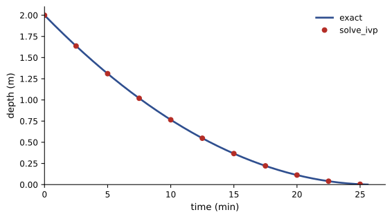
    print(f"  after {t_min:2d} min the depth is about {sol.y[0][i]:.2f} m")

Numerical: 25.6 min; exact: 25.6 min
  after  5 min the depth is about 1.31 m
  after 10 min the depth is about 0.77 m
  after 20 min the depth is about 0.11 m

The tank drains quickly at first and slowly at the end, because the outflow depends on the square root of the depth. The numerical result matches the exact solution, which exists for this simple case and is the reason it was chosen: always test a solver on a problem with a known answer before trusting it on one without. The same set-up, with more terms in the equation (inflow, pumps, variable cross-section), models stormwater ponds, reservoirs and process tanks for which no exact solution exists. Euler's method from Lesson 5 would also work here, but would need a carefully chosen fixed step and give no error control.

Fitting models to data

Lesson 5 fitted a straight line with np.polyfit. Many engineering models are not straight lines or polynomials: exponential decay, power laws, saturation curves. scipy.optimize.curve_fit fits any model function to data by nonlinear least squares, starting from initial guesses p0, and returns the best parameters and their covariance matrix, from which standard errors and confidence intervals follow (ENGG-160).

import numpy as np
from scipy.optimize import curve_fit

# Cooling of a casting: temperature (C) against time (min)
t = np.array([0, 5, 10, 15, 20, 30, 40, 60])
T = np.array([612, 461, 352, 271, 212, 136, 94, 55])
T_room = 22.0

def model(t, T0, k):
    return T_room + (T0 - T_room) * np.exp(-k * t)    # Newton cooling

(T0, k), cov = curve_fit(model, t, T, p0=[600, 0.05])
se_k = np.sqrt(cov[1, 1])
print(f"T0 = {T0:.0f} C, k = {k:.4f} per min (+/- {1.96 * se_k:.4f}, 95%)")
print(f"Time constant {1 / k:.1f} min; time to reach 100 C {np.log((T0 - T_room) / (100 - T_room)) / k:.1f} min")
print("Largest residual:", np.round(np.abs(T - model(t, T0, k)).max(), 1), "C")

T0 = 606 C, k = 0.0556 per min (+/- 0.0023, 95%)
Time constant 18.0 min; time to reach 100 C 36.2 min
Largest residual: 12.2 C

The fit gives a cooling constant of 0.056 per minute (a time constant of 18 minutes), with a 95 % confidence interval of about ±4 %, and predicts that the casting reaches 100 °C, cool enough to handle with gloves for shake-out, after about 36 minutes. The largest residual, 12 °C, is worth a look: early in cooling, radiation is significant at 600 °C and the simple exponential model is only approximate. Residual patterns, as in Lesson 8, show where a model falls short.

Two cautions apply to nonlinear fitting. Poor initial guesses can lead the fit to a wrong local minimum or fail to converge, so choose p0 from physical reasoning or a plot. And a good fit within the range of data does not justify extrapolating far beyond it.

Optimization

scipy.optimize.minimize finds the minimum of a function of several variables, with optional bounds and constraints, and minimize_scalar handles one variable. Engineers use these for design optimization (lightest beam meeting stress and deflection limits, cheapest pipe diameter balancing capital and pumping cost), for parameter estimation, and for operating decisions. scipy.optimize.linprog solves linear programs, such as allocating production or blending materials at least cost. MATH-300 and AI-310 develop these methods.

Monte Carlo simulation

Most engineering inputs are uncertain: loads, material strengths, dimensions, costs, durations, weather. A single calculation with typical values gives a typical answer but says nothing about the spread or the chance of an extreme outcome. Monte Carlo simulation, named after the casino, propagates uncertainty by brute force: draw random values of every uncertain input from its probability distribution, compute the output, repeat thousands or millions of times, and examine the distribution of results. With NumPy, all the samples can be drawn and computed at once as arrays.

import math
import numpy as np

rng = np.random.default_rng(2026)
N = 1_000_000
# Resistance of a member (kN m): normal, mean 420, CoV 10 percent
R = rng.normal(420, 42, N)
# Load effect: dead (normal) plus snow (Gumbel, a typical model for annual maxima)
D = rng.normal(90, 9, N)
S = rng.gumbel(80, 22, N)
Q = D + S
fails = R < Q
pf = fails.mean()
print(f"Mean load effect {Q.mean():.0f} kN m; failures {fails.sum()} of {N:,}")
print(f"Probability of failure per year {pf:.2e} (about 1 in {1 / pf:,.0f})")
se = math.sqrt(pf * (1 - pf) / N)
print(f"Standard error of the estimate {se:.1e} ({se / pf:.0%} of the estimate)")
M = R - Q                                         # safety margin
beta = M.mean() / M.std()
print(f"Reliability index assuming the margin is normal: {beta:.2f}")

Mean load effect 183 kN m; failures 83 of 1,000,000
Probability of failure per year 8.30e-05 (about 1 in 12,048)
Standard error of the estimate 9.1e-06 (11% of the estimate)
Reliability index assuming the margin is normal: 4.62

A member with a mean resistance of 420 kN·m carries a mean load effect of only 183 kN·m, yet the simulation finds that resistance falls below load in about 1 in 12,000 years. The reliability index computed by assuming the safety margin R − Q is normal is 4.62, which would correspond to a probability of only about 2 in a million: forty times smaller. The difference comes from the snow load's Gumbel distribution, whose long upper tail produces rare heavy snowfalls that a normal distribution would not. Tails matter, and Monte Carlo captures them without needing a formula. Modern structural codes are calibrated so that members achieve target reliability indices using this kind of analysis, with more refined statistical models.

The precision of a Monte Carlo estimate improves only with the square root of the number of samples: the standard error of an estimated probability p from N samples is √(p(1 − p)/N). With a million samples and 83 failures, the estimate is good to about 11 %; estimating probabilities of one in a million would need hundreds of millions of samples or smarter sampling methods (importance sampling). Always report the standard error, and fix the random seed so results can be reproduced.