Simulation and design verification

Between the preliminary and critical design reviews, the team had six weeks to show that their designs would work before any money was spent on boards. Hardware is slow and expensive to change; a simulation or a calculation is not. This lesson covers how the team used analysis and simulation to verify the designs: the levels of modelling, circuit simulation of the converter, worst-case and Monte Carlo analysis of a measurement chain, a design failure modes and effects analysis, and the critical design review where it all came together.

Verification and validation

Two words are used carefully in engineering. Verification asks whether the design meets its specified requirements: did we build the thing right? Validation asks whether the requirements, and the product, actually meet the client's need: did we build the right thing? A converter that reaches 97.5 % efficiency has been verified against R5; whether the canopy keeps the trucks storm-ready in a real winter is a validation question that only operation can fully answer. Analysis and simulation are verification tools, and they are only as good as the models behind them.

Levels of modelling

The team used models at several levels of detail, choosing the simplest that could answer each question. Hand calculations and short programs, like those in earlier lessons, sized components and checked energy. Averaged models, which replace switching with its average effect, were used for the control loops, because they run quickly and show the dynamics that matter for stability. Switching-level circuit simulation, in a SPICE-type simulator with the manufacturer's device models, was used for the power stage, to see voltage overshoot, dead-time behaviour and switching losses that averaged models hide. A thermal model of the heat sink and enclosure estimated temperatures. And the hourly energy model checked the whole system against the requirements over a day.

Every model has limits, and a team should be able to say what each one leaves out. The averaged converter model ignores switching ripple and assumes continuous conduction. The device models from manufacturers are good for switching transitions at typical conditions but less reliable at temperature extremes. The hourly energy model ignores weather variability within a season. Writing these limits next to each result is part of verification, because a reviewer needs to know how far to trust it.

Simulating the power stage

Aisha's switching simulation of one converter leg included the MOSFET models, the gate driver's output resistance and the gate resistor, an estimate of the loop inductance from her planned layout, the bus capacitors with their equivalent series resistance and inductance, and the inductor. The first run showed drain-source overshoot of about 90 V at turn-off with the planned 3 Ω gate resistor, which left 160 V of margin to the 650 V rating, acceptable but less than she wanted. Raising the gate resistor slowed the switching edge and reduced overshoot, but increased switching loss. She settled on 4.7 Ω, which cut the overshoot to about 60 V at a cost of about 2 W more switching loss across the four devices.

This is a typical trade. Faster switching means lower switching loss but more overshoot, more ringing and more electromagnetic interference. The simulation let Aisha quantify it before layout. Her logbook recorded the change, but, as lesson 10 reveals, she did not update the loss estimate in the report, a small slip that caught up with her later.

Worst-case and statistical analysis

Every component has a tolerance, and a design must work across the range of values its components might have, at the temperatures it will see. Three methods are common. Worst-case analysis sets every tolerance at its limit in the most damaging direction and checks the requirement still holds; it is simple and conservative, sometimes so conservative that it forces expensive parts. Root-sum-square analysis assumes errors are independent and combines them as the square root of the sum of squares, which is less pessimistic but still a single number. Monte Carlo analysis draws random values for each component from its distribution many thousands of times and looks at the spread of results, which shows not only the range but how likely each part of it is.

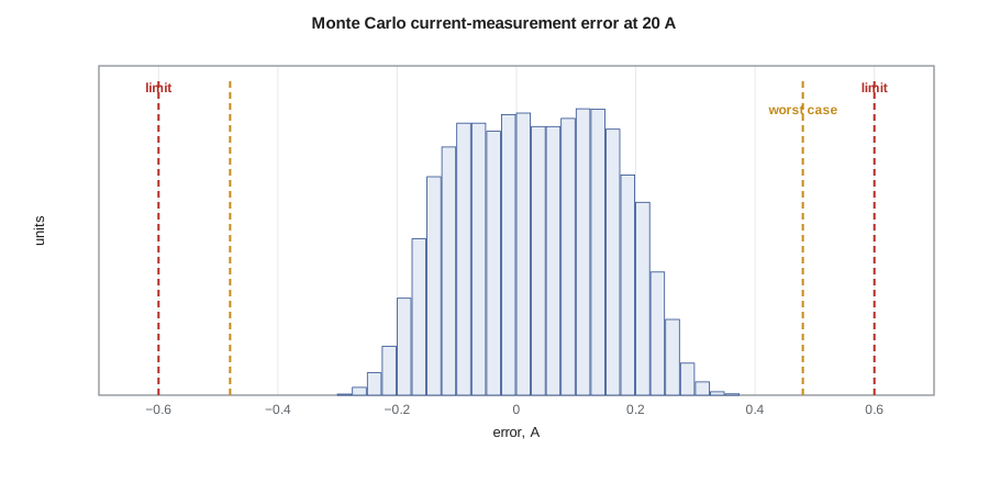
Mateo applied all three to the converter's battery current measurement, which the site controller uses for energy accounting and the firmware uses for protection. The chain is a 1 mΩ shunt resistor, an amplifier with a gain of 20, and a 12-bit analog-to-digital converter with a 2.5 V reference. The requirement he derived was an error within 2 % of the 30 A full scale, 0.6 A.

# Battery current measurement chain: worst case, root-sum-square and Monte Carlo against a 2 % requirement
import random, statistics, math
I_FS = 30.0                                       # full-scale current, A
R_SH, G_AMP, V_REF, OFFS = 0.001, 20.0, 2.5, 0.0  # nominal shunt ohms, amplifier gain, ADC reference, offset V
tol = {'shunt': 0.01, 'gain': 0.005, 'vref': 0.002}   # +/- fractional limits
OFF_MAX, TEMPCO, DT = 0.0015, 50e-6, 60.0          # amplifier offset (V at output), shunt ppm/K, self-heating K
def measured(i, rs, g, vr, off):
    v = i * rs * g + off                          # amplifier output
    code = round(v / vr * 4095)                   # 12-bit ADC
    return code / 4095 * V_REF / (R_SH * G_AMP)   # firmware uses nominal values
true = 20.0
worst = max(abs(measured(true, R_SH * (1 + a * tol['shunt']) * (1 + TEMPCO * DT), G_AMP * (1 + b * tol['gain']),
                         V_REF * (1 + c * tol['vref']), d * OFF_MAX) - true)
            for a in (-1, 1) for b in (-1, 1) for c in (-1, 1) for d in (-1, 1))
rss = math.sqrt(tol['shunt'] ** 2 + tol['gain'] ** 2 + tol['vref'] ** 2 + (TEMPCO * DT) ** 2) * true + OFF_MAX / (R_SH * G_AMP)
random.seed(4)
err = []
for _ in range(20000):
    rs = R_SH * (1 + random.uniform(-1, 1) * tol['shunt']) * (1 + TEMPCO * random.uniform(0, DT))
    g = G_AMP * (1 + random.gauss(0, tol['gain'] / 3)); vr = V_REF * (1 + random.gauss(0, tol['vref'] / 3))
    err.append(measured(true, rs, g, vr, random.gauss(0, OFF_MAX / 3)) - true)
err.sort()
lim = 0.02 * I_FS
p_out = sum(abs(e) > lim for e in err) / len(err) * 100
print(f"requirement: error within {lim:.2f} A (2 % of full scale) at {true:.0f} A")
print(f"worst case {worst:.3f} A, RSS estimate {rss:.3f} A")
print(f"Monte Carlo: mean {statistics.mean(err):+.3f} A, 99.7 % of units within {max(abs(err[30]), abs(err[-31])):.3f} A, outside limit {p_out:.2f} %")

requirement: error within 0.60 A (2 % of full scale) at 20 A
worst case 0.482 A, RSS estimate 0.310 A
Monte Carlo: mean +0.031 A, 99.7 % of units within 0.330 A, outside limit 0.00 %

The worst case gives 0.48 A of error at 20 A, inside the 0.6 A requirement, so the design passes on the most conservative method without needing tighter parts. The root-sum-square estimate is 0.31 A, and the Monte Carlo result shows 99.7 % of units within about 0.33 A, with a small positive bias. The bias comes from the shunt's self-heating: its resistance rises with temperature, always in the same direction, so it does not average out. Mateo added a temperature correction in firmware using the board's temperature sensor, which halved the bias, and recorded that a single-point calibration at the end of production would remove most of the remaining error if a later version needed tighter accuracy.

Design failure modes and effects analysis

Simulation checks that a design works when its parts behave. A failure modes and effects analysis (FMEA) asks what happens when they do not. For each component or function, the team listed how it could fail, the effect on the system, the cause, the controls already in the design that prevent or detect it, and a rating of severity, occurrence and detection. Hannah ran the FMEA as a two-hour workshop with all four members and Ravi, who had seen many real failures at Larchmont. Recent guidance on FMEA, such as the 2019 handbook published jointly by the automotive industry groups AIAG and VDA, prioritizes actions by severity first rather than by a single multiplied number, and the team followed that approach.

Three findings changed the design. A MOSFET failing short in one leg would short the bus through the other device of the same leg on its next turn-on; the gate driver's desaturation protection catches this, but only if it is enabled before the first switching cycle, so Mateo changed the start-up sequence. The pre-charge resistor could overheat if the contactor failed to close and the firmware kept retrying; a retry limit and a thermal fuse were added. And loss of the battery management system's communication could leave the converter charging a battery whose cells it could not see; the converter now stops within one second of losing that link. Each finding went into the risk register with an owner and was verified in testing.

Checking the analysis itself

Analysis can be wrong in ways that look right. The team used three checks on every important calculation. First, a second person repeated it independently, without looking at the first result, using a different method where one existed: Hannah checked Aisha's loss estimate with a spreadsheet built from the same datasheets, and found a factor of two error in the capacitor ripple current that Aisha's program had made by using the per-phase rather than the total current. Second, every result was compared with a simple bound or rule of thumb: a 6 kW SiC converter at this frequency typically achieves 98 to 99 % efficiency, so a prediction of 99.6 % would have been a warning sign. Third, units were carried through every step, in calculations and in code comments, which catches the most common errors before they propagate.

Analysing the full system

Hannah and Leo applied the same thinking to the full-size canopy design, at a coarser level. What if the zero-export relay fails? The inverter's own export limit still works, and the relay's self-test reports its failure to SCADA. What if the battery is unavailable on a winter night? The controller falls back to grid-only charging within the 60 kW limit. Over a thirteen-hour night that still delivers the fleet's 360 kWh, because 60 kW for thirteen hours is far more than the vehicles need, but the midday top-up becomes slower and there is no storm reserve, so the operations centre is alerted. What if a storm outage lasts longer than the battery can cover? The two storm trucks are prioritized, and the canopy's solar can extend the reserve in daylight. The team documented each scenario and its outcome, which became the operations section of the handover manual.

The critical design review

The CDR in week fifteen was the gate before hardware. The team presented the detailed converter and controller designs, the simulation and analysis results with their limits, the FMEA, the full-size canopy drawings, the bill of materials, the test plan and an updated schedule and budget. The review panel, Professor Gagnon, Marguerite, Nadine and a power electronics engineer from Cedarline, had read the package in advance and came with questions.

The panel approved the controller and the canopy design, and approved the converter with two conditions. The Cedarline reviewer noticed that the current-sense amplifier had been simulated with its common-mode voltage at 0 V, while in the circuit the low-side shunt's common-mode voltage swings with switching noise; Mateo had to show the amplifier's common-mode rejection was adequate at 50 kHz before layout was released. And Nadine asked for the battery input fuse's rating to be checked against the battery's short-circuit current, not just its normal current. Both were closed within a week. Being sent back on details at a CDR is not a failure; it is what the review is for.