
ELE-350 · Lesson 3 of 12 · 24 min
Angle modulation: FM and PM
In amplitude modulation the message changes the size of the carrier. In angle modulation it changes the carrier's timing instead: its phase, or its instantaneous frequency. The amplitude stays constant, so noise and interference that change the amplitude can be removed with a limiter, and power amplifiers can run at their most efficient settings. Frequency modulation gave broadcast radio its high fidelity, it carries most land-mobile voice traffic, and its digital cousin, frequency-shift keying, is the modulation that Amara expects to use in the TLR-1. This lesson defines phase and frequency modulation, analyzes the spectrum with Bessel functions, introduces Carson's rule for bandwidth, and explains how FM signals are generated and demodulated.
Daniel brings a practical reason for the lesson. The city's maintenance crews still use narrowband FM handheld radios in a nearby band, and the cabinet will sit beside a traffic technician's truck radio during every service visit. The TLR-1 receiver must not be disturbed by a 5 W FM transmitter a metre away, and Amara needs to know how wide such a signal really is. Leo also has an old FM broadcast receiver on the bench, and its circuit will serve as the example receiver in lesson 4.
Instantaneous phase and frequency
Write a carrier as A_c cos θ(t), where θ(t) is the total angle. For an unmodulated carrier, θ(t) = 2πf_c t, and the angle grows at a constant rate. The instantaneous frequency is defined as the rate of change of the angle divided by 2π. Angle modulation makes the angle depart from the steady ramp in step with the message.
In phase modulation (PM), the phase deviation is proportional to the message: θ(t) = 2πf_c t + k_p m(t), with k_p in radians per volt. In frequency modulation (FM), the instantaneous frequency deviation is proportional to the message: f_i(t) = f_c + k_f m(t), with k_f in hertz per volt, so the phase is proportional to the integral of the message.
The two are closely related. FM of a message is PM of its integral, and PM of a message is FM of its derivative. A phase modulator preceded by an integrator is an FM transmitter, and that is exactly how the Armstrong method below works. For a single tone the only visible difference is that the PM frequency deviation grows with the tone frequency, while the FM deviation does not.
Frequency deviation and modulation index
For FM by a tone m(t) = A_m cos(2πf_m t), the instantaneous frequency swings by Δf = k_f A_m either side of the carrier. The peak frequency deviation Δf is set by the message amplitude, not its frequency. The phase swings by β = Δf/f_m radians, and β is the FM modulation index. A loud low note produces a large β; a quiet high note a small one.
For a general message, the analogous figure is the deviation ratio D = Δf/W, where Δf is the peak deviation and W is the message bandwidth. FM broadcasting in North America uses a peak deviation of 75 kHz for an audio bandwidth of 15 kHz, so D = 5. Narrowband land-mobile FM on 12.5 kHz channels typically uses about 2.5 kHz deviation for voice up to 3 kHz, so D is under 1.
The spectrum of FM
Angle modulation is not linear. Doubling the message does not double the spectrum, and the spectrum of a sum is not the sum of the spectra. For a single tone, though, the spectrum can be found exactly. The term e^(jβ sin ω_m t) is periodic and can be expanded in a Fourier series whose coefficients are Bessel functions of the first kind, J_n(β). The FM signal is then a carrier and an infinite set of sidebands spaced f_m apart.
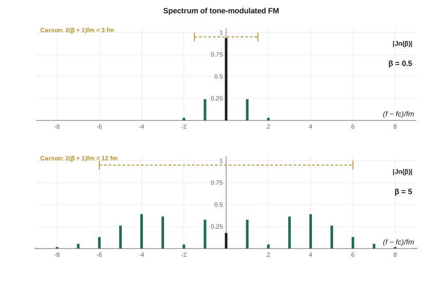
Three properties follow from the Bessel functions. First, the total power is always A_c²/2, whatever β is; modulation only redistributes it, and the carrier component J₀(β) shrinks as β grows. It falls to zero at β = 2.405, 5.52 and other zeros of J₀, a fact used to calibrate deviation meters: raise the tone level until the carrier line vanishes on a spectrum analyzer, and β is then exactly 2.405. Second, for small β only J₀ and J₁ are significant, so narrowband FM has a carrier and two sidebands like AM, but with the sidebands in quadrature with the carrier, which is why it has almost no amplitude variation. Third, the sideband amplitudes drop rapidly once n exceeds β + 1. That observation leads to the most widely used rule in FM work.
Carson's rule
Carson's rule estimates the bandwidth that holds about 98 percent of the power of an FM signal. For a tone it counts β + 1 sideband pairs; for a general message, it uses the peak deviation and the highest message frequency.
For FM broadcasting, B_T ≈ 2(75 + 15) = 180 kHz, which fits the 200 kHz channel spacing. For the city's narrowband handhelds, B_T ≈ 2(2.5 + 3) = 11 kHz, inside the 12.5 kHz channel. Carson's rule underestimates slightly for intermediate values of D, and filters in real equipment are designed with a margin, but it is accurate enough for planning. Two limits are worth remembering. When D is very small, B_T approaches 2W, the same as AM. When D is large, B_T approaches 2Δf, because the instantaneous frequency simply sweeps across the band.
Worked problem
Bandwidth of three FM signals
Find the Carson bandwidth and modulation index for: an FM broadcast station with Δf = 75 kHz and W = 15 kHz; a land-mobile handheld with Δf = 2.5 kHz and W = 3 kHz; and a 1 kHz test tone at Δf = 2.405 kHz.
Show solution
- \[\text{Broadcast: } D = 75/15 = 5, \quad B_T = 2(75 + 15) = 180\ \text{kHz}\]
- \[\text{Handheld: } D = 2.5/3 = 0.83, \quad B_T = 2(2.5 + 3) = 11\ \text{kHz}\]
- \[\text{Test tone: } \beta = 2.405/1 = 2.405, \quad B_T = 2(2.405 + 1) = 6.81\ \text{kHz}\]
Answer: The broadcast signal is sixteen times wider than the handheld one. The test tone's β is the first zero of J₀, so its carrier line disappears, a useful check that Leo's signal generator deviation is calibrated.
import math
def J(n, x, terms=40):        # Bessel function of the first kind, power series
    return sum((-1)**k * (x/2)**(2*k + n) / (math.factorial(k) * math.factorial(k + n)) for k in range(terms))
for beta in (0.5, 1.0, 2.405, 5.0):
    print(f"beta = {beta}:")
    print("   " + "  ".join(f"J{n}={J(n, beta):+.3f}" for n in range(0, 7)))
    nc = int(beta + 1)                     # sideband pairs inside Carson's bandwidth
    p = J(0, beta)**2 + 2 * sum(J(n, beta)**2 for n in range(1, nc + 1))
    print(f"   Carson pairs = {nc}, power inside = {100*p:.1f} %")
for name, df, W in (('broadcast', 75e3, 15e3), ('handheld', 2.5e3, 3e3)):
print(f"{name}: D = {df/W:.2f}, Carson bandwidth = {2*(df + W)/1e3:.1f} kHz")beta = 0.5: J0=+0.938 J1=+0.242 J2=+0.031 J3=+0.003 J4=+0.000 J5=+0.000 J6=+0.000 Carson pairs = 1, power inside = 99.8 % beta = 1.0: J0=+0.765 J1=+0.440 J2=+0.115 J3=+0.020 J4=+0.002 J5=+0.000 J6=+0.000 Carson pairs = 2, power inside = 99.9 % beta = 2.405: J0=-0.000 J1=+0.519 J2=+0.432 J3=+0.199 J4=+0.065 J5=+0.016 J6=+0.003 Carson pairs = 3, power inside = 99.1 % beta = 5.0: J0=-0.178 J1=-0.328 J2=+0.047 J3=+0.365 J4=+0.391 J5=+0.261 J6=+0.131 Carson pairs = 6, power inside = 99.4 % broadcast: D = 5.00, Carson bandwidth = 180.0 kHz handheld: D = 0.83, Carson bandwidth = 11.0 kHz
The output confirms the carrier null at β = 2.405 and shows that the sidebands inside Carson's bandwidth hold more than 99 percent of the power for these tones; the 98 percent usually quoted is a conservative round figure that also covers messages other than a single tone. The rule is a planning estimate; a spectrum mask in the regulations, not Carson's rule, decides whether a transmitter is legal.
Generating FM
The direct method uses a voltage-controlled oscillator. A varactor diode, whose capacitance falls as its reverse bias rises, is part of the tank circuit of an LC oscillator, and the message is added to its bias. The oscillator's frequency then follows the message. Direct FM is simple and can reach large deviations, but the centre frequency of a free-running LC oscillator drifts with temperature, so practical transmitters put the VCO inside a phase-locked loop referenced to a crystal. The loop is made slow enough not to follow the audio, but fast enough to correct drift.
The indirect, or Armstrong, method starts with narrowband FM made by a phase modulator, with the message integrated first, at a low carrier frequency where a crystal oscillator is stable. Because narrowband FM is almost the same as DSB-SC added to a carrier in quadrature, it can be built from a balanced modulator and a 90° phase shift. Frequency multipliers then raise both the carrier and the deviation by the same factor. A multiplier is a nonlinear stage, such as a transistor driven hard, followed by a filter that keeps the nth harmonic. Multiplying the frequency by n multiplies the deviation by n too, and mixing with a local oscillator then moves the carrier without changing the deviation. Armstrong's method was how wideband FM was first made stable enough for broadcasting.
Demodulating FM
An FM demodulator must produce an output proportional to the instantaneous frequency. The textbook circuit is the discriminator: a differentiator, which turns frequency variation into amplitude variation because the derivative of A_c cos θ(t) has amplitude A_c dθ/dt, followed by an envelope detector. Since any amplitude variation of the input would also appear at the output, a limiter is placed first; it clips the signal hard so that only the zero crossings, which carry the frequency information, remain. Practical analog receivers used a slope detector on a tuned circuit, the balanced Foster-Seeley and ratio detectors, or the quadrature detector in integrated FM receivers, which multiplies the signal by a copy delayed through a phase-shift network.
Modern receivers favour the phase-locked loop and its digital equivalents. A PLL locked to the incoming signal must move its VCO to follow the input frequency, so the VCO control voltage is the demodulated message. In a software or digital receiver, the signal is converted to in-phase and quadrature samples I and Q, the phase is computed as θ = atan2(Q, I), and the frequency is the difference between successive phases. The same arithmetic demodulates the FSK of the TLR-1.
Noise, the FM advantage and the threshold
Noise added to an FM signal disturbs its phase. At the discriminator output, the noise is shaped: phase noise is converted to frequency noise by differentiation, so its spectrum rises with frequency, growing as f². Meanwhile the wanted output grows with deviation. Above a certain input SNR, the result is that wideband FM trades bandwidth for output quality: for a tone, the output SNR improves over a baseband system with the same received power by a factor of 3β²/2, and with β = 5 that is about 16 dB, before de-emphasis adds more.
Because the output noise rises with frequency, FM systems boost the high audio frequencies before modulation, called pre-emphasis, and cut them by the same amount after demodulation, called de-emphasis. The cut lowers the high-frequency noise along with the boosted signal. North American FM broadcasting uses a 75 µs time constant, a corner near 2.1 kHz; much of the world uses 50 µs.
The advantage has a limit. When the input SNR falls below about 10 dB, noise occasionally swings the phase through a full 2π, producing clicks at the output, and the output SNR collapses much faster than the input. This is the FM threshold, and below it FM is worse than AM. Narrowband FM has a lower threshold, which is one reason mobile radio uses it. A related property, the capture effect, makes an FM receiver lock onto the stronger of two signals on the same frequency and almost completely suppress the weaker if the difference is a few dB. That is good for mobile radio and is also part of why the TLR-1, if it uses constant-envelope FSK, will tolerate a weak interferer well.
| Property | AM | Narrowband FM | Wideband FM |
|---|---|---|---|
| Bandwidth | 2W | about 2W | 2(Δf + W), several times 2W |
| Envelope | Follows the message | Constant | Constant |
| Amplifier | Must be linear | Can be saturated, efficient | Can be saturated, efficient |
| Noise performance | Output SNR equals baseband | Similar to AM above threshold | Large improvement above threshold |
| Weak points | Wastes carrier power | Threshold, capture | Bandwidth, threshold |
Stereo FM: a system of everything so far
FM stereo broadcasting packs three of this course's ideas into one signal. The sum of the left and right channels, L + R, is sent at baseband from 30 Hz to 15 kHz, so mono receivers work unchanged. The difference L − R is sent as DSB-SC on a 38 kHz subcarrier, occupying 23 to 53 kHz. A 19 kHz pilot tone, exactly half the subcarrier frequency, lets the receiver regenerate the suppressed carrier coherently by doubling it. A digital data subcarrier at 57 kHz often carries station names and traffic messages. The whole composite baseband then frequency-modulates the main carrier. A receiver that decodes stereo is performing frequency division multiplexing, coherent demodulation and carrier recovery in one small chip.
Common mistakes
MistakeCalling β the frequency deviation.
Insteadβ = Δf/f_m is in radians; Δf is the frequency deviation in hertz.
MistakeAssuming FM bandwidth is just 2Δf.
InsteadCarson's rule adds the message bandwidth: B_T ≈ 2(Δf + W), which matters when D is small.
MistakeExpecting a frequency multiplier to leave deviation unchanged.
InsteadMultiplying frequency by n multiplies deviation by n; only mixing shifts the carrier without changing deviation.
MistakeThinking FM always beats AM in noise.
InsteadBelow the threshold, near 10 dB input SNR, FM output degrades sharply and can be worse than AM.
Summary and key terms
- PM varies phase in proportion to the message; FM varies instantaneous frequency, so its phase is the integral of the message.
- For tone FM, β = Δf/f_m; the spectrum has sidebands at f_c ± nf_m with amplitudes J_n(β), and total power is constant.
- Carson's rule, B_T ≈ 2(Δf + W), holds about 98 percent of the power.
- FM is generated directly with a VCO in a PLL or indirectly with a phase modulator and frequency multipliers.
- Demodulators measure instantaneous frequency: discriminators, quadrature detectors, PLLs or the phase difference of I/Q samples.
- Above threshold, wideband FM trades bandwidth for output SNR; pre-emphasis helps; below about 10 dB input SNR the advantage collapses.
- Frequency deviation
- The peak difference between the instantaneous frequency and the carrier frequency.
- Modulation index (FM)
- For tone FM, the ratio of peak frequency deviation to tone frequency; the peak phase deviation in radians.
- Deviation ratio
- Peak deviation divided by the highest message frequency.
- Carson's rule
- The estimate 2(Δf + W) for the bandwidth holding about 98 percent of an FM signal's power.
- Limiter
- A circuit that removes amplitude variation by clipping, leaving the zero crossings.
- Pre-emphasis
- Boosting high message frequencies before modulation so that de-emphasis can reduce high-frequency noise.
- FM threshold
- The input SNR below which FM output quality falls sharply.
- Capture effect
- The tendency of an FM receiver to suppress the weaker of two co-channel signals.
Practice problems
Work each problem on paper first, then reveal the answer to check.
A 2 kHz tone produces a peak deviation of 6 kHz. Find β and the Carson bandwidth.
Show answer
β = 3; B_T = 2(6 + 2) = 16 kHz.
A VCO has a sensitivity of 15 kHz/V. What peak deviation does a 0.4 V peak message give?
Show answer
6 kHz.
An FM signal at 10 MHz with 2 kHz deviation passes through a ×9 multiplier. Give the new carrier and deviation.
Show answer
90 MHz and 18 kHz.
Why does a limiter come before a discriminator?
Show answer
The discriminator responds to amplitude as well as frequency; the limiter removes amplitude variation from noise and fading.
Using J₀(1) ≈ 0.765, what fraction of power remains in the carrier at β = 1?
Show answer
0.765² ≈ 0.585, about 59 percent.
For narrowband FM with Δf = 5 kHz and W = 3 kHz, what does Carson's rule give, and would it fit a 12.5 kHz channel?
Show answer
16 kHz; it would not fit, which is why 12.5 kHz channels use about 2.5 kHz deviation.
Lesson quiz · 5 questions
Score 60% or more to complete this lesson.
Create a free account to save your progress, take quizzes and earn a certificate.