
ELE-340 · Lesson 6 of 12 · 23 min
Cascodes and wideband techniques
Lesson 5 showed that a common-emitter stage's bandwidth is usually limited not by its transistor but by the Miller multiplication of C_μ. The cure is to stop the collector of the gain transistor from swinging. The cascode does exactly that by stacking a common-base transistor on top of the common-emitter one: the CE transistor still provides the transconductance, the CB transistor passes the signal current to the load, and the CE collector sits at an almost constant voltage. The result has the gain of a CE stage, a much wider bandwidth and a far higher output resistance. This lesson analyzes the cascode, then surveys the other ways designers extend bandwidth: buffering the source, using CC-CB pairs, local feedback, inductive peaking and careful distribution of gain among stages.
The application is on Leo's bench. Cedarline's production test fixture for the APS-2 digitizes test signals at 10 million samples per second, and the fixture's front end must amplify a signal from a 1 kΩ test point by about 100 with a bandwidth of at least 2 MHz, so that the fast edges of the controller's synchronization pulses are measured faithfully. A single CE stage, as lesson 5 showed, falls short.
The cascode
In the BJT cascode, Q1 is a common-emitter stage whose collector connects to the emitter of Q2. The base of Q2 is held at a fixed DC voltage V_BIAS and bypassed to signal ground, so Q2 is a common-base stage. The signal current g_m1 v_be1 from Q1 enters Q2's emitter, which presents only r_e2 ≈ 1/g_m2, and emerges almost unchanged from Q2's collector into the load R_L. Since both transistors carry the same current, g_m1 = g_m2, and the voltage gain from Q1's base to its own collector is only about −g_m1 r_e2 ≈ −1. The Miller multiplication of C_μ1 is therefore about 2 instead of about 200.
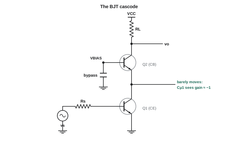
Three properties make the cascode valuable. Its gain with a resistor load equals that of the plain CE stage, because the signal current is the same. Its output resistance is huge, about β times r_o for a BJT and the intrinsic gain times r_o for a MOSFET, so with a cascoded current-source load a single stage can reach gains of tens of thousands; that is how telescopic and folded-cascode op amps get high gain in a single stage. And its bandwidth is wide, because the Miller effect is gone. The costs are an extra transistor, a bias voltage for Q2's base, and headroom: Q1 needs its own V_CE above saturation, so the output cannot swing as low as a single stage's.
Worked problem
Time constants of the cascode
Rebuild the lesson 5 stage as a cascode, with Q1 and Q2 identical (1 mA, β = 100, C_π = 16 pF, C_μ = 2 pF), the same R_s' = 721 Ω, R_L' = 5 kΩ and C_L = 5 pF. Estimate f_H by open-circuit time constants.
Show solution
- Q1's collector sees r_e2 ≈ 25.9 Ω, so its base-to-collector gain is about −1:
- \[\tau_{\pi 1} = 721 \times 16\ \text{pF} = 11.5\ \text{ns} \qquad \tau_{\mu 1} = \big[721(1 + 1) + 26\big] \times 2\ \text{pF} = 2.9\ \text{ns}\]
- \[\tau_{\pi 2} \approx 26 \times 16\ \text{pF} = 0.4\ \text{ns} \qquad \tau_{\mu 2} = 5\ \text{k} \times 2\ \text{pF} = 10\ \text{ns} \qquad \tau_L = 5\ \text{k} \times 5\ \text{pF} = 25\ \text{ns}\]
- \[\sum \tau \approx 49.9\ \text{ns} \qquad f_H \approx \frac{1}{2\pi \times 49.9\ \text{ns}} \approx 3.2\ \text{MHz}\]
Answer: The cascode keeps the mid-band gain of about −139 but raises the upper corner from about 487 kHz to about 3.2 MHz, a factor of 6.5. The bottleneck has moved: the largest time constant is now the output node, R_L'(C_μ2 + C_L) = 35 ns, so further improvement needs a smaller load capacitance, a lower R_L' with more current, or a follower to isolate the load.
Other wideband combinations
The cascode is one of several two-transistor answers to the Miller problem, each attacking a different term in the time-constant sum:
| Combination | Idea | Which time constant it reduces | Typical use |
|---|---|---|---|
| Cascode (CE-CB) | CB transistor holds the CE collector still | C_μ1 term: R_s'(1 + g_m R_L') becomes about 2R_s' | Wideband gain stages, high-gain op amp stages |
| CC-CE | Input follower drives the CE base from a low resistance | R_s' falls to about R_s/β + r_e | High source resistance, such as sensors and photodiodes |
| CC-CB (emitter-coupled pair) | Follower drives a grounded-base stage; no inverting gain at any base | Removes Miller multiplication entirely | Limiting amplifiers, wideband differential stages |
| CE-CC | Output follower isolates the load | C_L term: R_L' seen by C_L falls to about r_e + R_L/β | Driving cables and capacitive loads |
| Local feedback pairs | Series or shunt feedback trades gain for bandwidth | Reduces effective gain and resistances at each node | Broadband amplifier blocks |
For the test fixture, the obvious combination is a cascode followed by an emitter follower: the cascode removes the Miller term, and the follower stops the digitizer's input capacitance and the cable from loading the 5 kΩ output node. In integrated circuits the folded cascode does the same job at lower supply voltages by using a pnp or PMOS CB transistor, so that the output can swing higher.
Inductive peaking
When the output node limits bandwidth, a small inductor in series with the load resistor helps. At low frequencies it does nothing; at high frequencies its rising impedance raises the load impedance just as the load capacitance starts to shunt it, so the gain stays up longer. With an inductance of about 0.4R²C, called shunt peaking, the bandwidth of an RC-limited node increases by roughly 1.7 times with a flat response, and more if some overshoot is acceptable. Peaking was invented for television video amplifiers and survives in high-speed integrated circuits for optical links, where on-chip inductors are cheap. It is rarely worth the trouble in a 2 MHz design like Leo's.
Spreading gain across stages
A large gain is sometimes better split among several stages, but bandwidth shrinks as identical stages are cascaded, because their attenuations multiply. For n identical single-pole stages, each with bandwidth f_1, the overall bandwidth is
so two stages give 64 percent of one stage's bandwidth, three give 51 percent and four 43 percent. Against that, each stage needs only the nth root of the total gain, and for a fixed gain-bandwidth product per stage, lower gain means proportionally more bandwidth. The balance has an optimum. With a total gain G and a per-stage gain-bandwidth product GBW, n stages of gain G^(1/n) each have bandwidth GBW/G^(1/n), and the cascade has GBW/G^(1/n) × √(2^(1/n) − 1). The code below finds the best n for Leo's requirement.
import math
VT = 0.02585
# Cascode time constants for the lesson 5 example
gm = 1e-3 / VT; beta = 100
Cpi, Cmu, CL = 16e-12, 2e-12, 5e-12
Rs, RL = 721.0, 5e3
re2 = 1 / gm
ce = Rs * Cpi + (Rs * (1 + gm * RL) + RL) * Cmu + RL * CL
cas = Rs * Cpi + (Rs * (1 + gm * re2) + re2) * Cmu + re2 * Cpi + RL * Cmu + RL * CL
print(f"CE: sum of tau = {ce*1e9:.1f} ns, fH = {1/(2*math.pi*ce)/1e6:.2f} MHz")
print(f"cascode: sum of tau = {cas*1e9:.1f} ns, fH = {1/(2*math.pi*cas)/1e6:.2f} MHz")
# Bandwidth of n identical stages
for n in (1, 2, 3, 4):
    print(f"{n} identical stages: overall bandwidth = {math.sqrt(2**(1/n)-1):.3f} x one stage")
# Optimum number of stages for a total gain of 100 with 60 MHz gain-bandwidth per stage
G, GBW = 100, 60e6
best = None
for n in range(1, 11):
    g = G ** (1 / n)
    bw = GBW / g * math.sqrt(2 ** (1 / n) - 1)
    print(f"n = {n}: gain per stage {g:6.2f}, overall bandwidth {bw/1e6:5.2f} MHz")
    if best is None or bw > best[1]:
        best = (n, bw)
print(f"best: {best[0]} stages, {best[1]/1e6:.2f} MHz")CE: sum of tau = 326.9 ns, fH = 0.49 MHz cascode: sum of tau = 49.9 ns, fH = 3.19 MHz 1 identical stages: overall bandwidth = 1.000 x one stage 2 identical stages: overall bandwidth = 0.644 x one stage 3 identical stages: overall bandwidth = 0.510 x one stage 4 identical stages: overall bandwidth = 0.435 x one stage n = 1: gain per stage 100.00, overall bandwidth 0.60 MHz n = 2: gain per stage 10.00, overall bandwidth 3.86 MHz n = 3: gain per stage 4.64, overall bandwidth 6.59 MHz n = 4: gain per stage 3.16, overall bandwidth 8.25 MHz n = 5: gain per stage 2.51, overall bandwidth 9.21 MHz n = 6: gain per stage 2.15, overall bandwidth 9.75 MHz n = 7: gain per stage 1.93, overall bandwidth 10.03 MHz n = 8: gain per stage 1.78, overall bandwidth 10.15 MHz n = 9: gain per stage 1.67, overall bandwidth 10.18 MHz n = 10: gain per stage 1.58, overall bandwidth 10.14 MHz best: 9 stages, 10.18 MHz
With 60 MHz of gain-bandwidth per stage, a single stage of gain 100 reaches only 0.6 MHz, two stages of gain 10 reach about 3.9 MHz, and three stages about 6.6 MHz. Each further stage helps less, and the theoretical optimum, near nine stages with a gain of only about 1.65 each, is useless in practice: every stage adds parts, power, noise and another chance of oscillation. Leo's requirement of 2 MHz is met comfortably by two stages. The general lesson is that splitting a large gain into two or three stages buys a great deal of bandwidth, and splitting it further buys little.
Worked problem
The fixture front end
Leo builds two cascode stages, each with a gain of about −10 and its own upper corner near 5 MHz, followed by an emitter follower driving the digitizer. Assuming single-pole stages and a follower with a corner far above, estimate the overall bandwidth and the 10–90 percent rise time of a step.
Show solution
- \[f_{H,2} = 5\ \text{MHz} \times \sqrt{2^{1/2} - 1} = 5 \times 0.644 \approx 3.2\ \text{MHz}\]
- \[t_r \approx \frac{0.35}{f_H} = \frac{0.35}{3.2\ \text{MHz}} \approx 109\ \text{ns}\]
Answer: The front end has an overall bandwidth near 3.2 MHz and a rise time near 110 ns, which is short compared with the 1 µs edges of the synchronization pulses the fixture must measure. The rule t_r ≈ 0.35/f_H holds for single-pole and similar responses and is the quickest way to translate bandwidth into what an oscilloscope will show.
Where wideband amplifiers go next
Beyond these techniques lie families of circuits designed for bandwidth first. Current-feedback op amps use a low-impedance inverting input and a transimpedance gain stage, so that their bandwidth depends only weakly on the closed-loop gain, unlike the fixed gain-bandwidth product of a voltage-feedback op amp. Distributed amplifiers spread the gain of several transistors along artificial transmission lines so that their capacitances become part of the lines. And radio-frequency amplifiers match their transistors to 50 Ω systems with tuned networks, trading bandwidth for gain at one frequency; ELE-455 takes that path. All of them build on the same insight as the cascode: find the capacitance that limits the response, and arrange the circuit so it no longer matters.
Common mistakes
MistakeAssuming a cascode increases the gain of a resistor-loaded stage.
InsteadWith the same R_L, the gain is the same; the cascode raises bandwidth and output resistance.
MistakeForgetting to bypass the cascode transistor's base.
InsteadAn unbypassed base adds impedance in the CB path and brings back gain and Miller effects.
MistakeCascading many identical stages without checking bandwidth.
Insteadn stages shrink bandwidth by √(2^(1/n) − 1); check the overall corner.
MistakeLeaving a high-impedance output node to drive a cable.
InsteadAdd a follower; the load capacitance otherwise becomes the bottleneck.
Summary and key terms
- The cascode stacks a CB transistor on a CE transistor, holding the CE collector nearly still.
- Its gain equals the CE stage's for the same load, but C_μ1 is multiplied by only about 2.
- Cascode output resistance is about βr_o (BJT) or g_m r_o² (MOSFET), enabling very high gain with active loads.
- CC-CE, CC-CB and CE-CC combinations attack the source, Miller and load time constants respectively.
- Shunt peaking with an inductor of about 0.4R²C extends an RC-limited node's bandwidth by roughly 1.7 times.
- n identical stages have bandwidth f₁√(2^(1/n) − 1); an optimum number of stages exists for a given total gain.
- Rise time is about 0.35/f_H for single-pole-like responses.
- Cascode
- A common-emitter (or common-source) stage followed by a common-base (or common-gate) stage.
- Folded cascode
- A cascode in which the common-base or common-gate transistor is of the opposite polarity, saving headroom.
- Shunt peaking
- Adding an inductor in series with a load resistor to extend the bandwidth of a capacitively loaded node.
- Bandwidth shrinkage
- The reduction of overall bandwidth when stages with similar corners are cascaded.
- Rise time
- The time a step response takes to rise from 10 to 90 percent of its final value.
- Current-feedback op amp
- An op amp with a low-impedance inverting input whose bandwidth depends weakly on closed-loop gain.
Practice problems
Work each problem on paper first, then reveal the answer to check.
In a BJT cascode with identical transistors, what is the approximate gain from Q1's base to Q1's collector?
Show answer
About −g_m1 r_e2 ≈ −1.
Find the output resistance of a BJT cascode with β = 120 and r_o = 80 kΩ.
Show answer
About 120 × 80 k = 9.6 MΩ.
Three identical stages each have a 6 MHz bandwidth. Find the overall bandwidth.
Show answer
6 × √(2^(1/3) − 1) = 6 × 0.510 ≈ 3.1 MHz.
An amplifier has a 20 MHz bandwidth. Estimate its 10–90 percent rise time.
Show answer
0.35/20 MHz = 17.5 ns.
An RC-limited node has R = 1 kΩ and C = 10 pF. What inductance gives shunt peaking near the flat-response value?
Show answer
0.4 × 10⁶ × 10⁻¹¹ = 4 µH.
Why is a follower placed after a cascode when driving a cable?
Show answer
The cascode's high-resistance output node would form a low-frequency pole with the cable capacitance.
Lesson quiz · 5 questions
Score 60% or more to complete this lesson.
Create a free account to save your progress, take quizzes and earn a certificate.