Sampling and aliasing

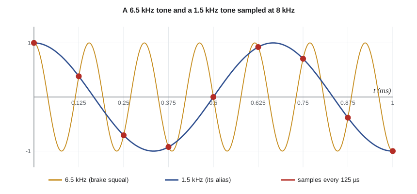
During field tests, Amara notices something odd in the accessible pedestrian signal's logs. Whenever a particular city bus stops at the corner, the noise detector reports a strong tone near 1.5 kHz, yet nobody standing at the corner hears anything at 1.5 kHz. What they hear is the bus's brakes squealing at about 6.5 kHz. The microcontroller samples the microphone 8,000 times a second, and a 6.5 kHz tone sampled at that rate produces exactly the same sequence of numbers as a 1.5 kHz tone. Once the samples are taken, no amount of clever processing can tell the two apart. This lesson explains why, states the sampling theorem that says how fast a signal must be sampled, and shows what the anti-aliasing filter from lesson 8 has to do.

Sampling in the frequency domain

An ideal sampler takes the value of x(t) every T seconds, giving x[n] = x(nT), with sampling frequency f_s = 1/T. To see what sampling does to the spectrum, model it as multiplying x(t) by an impulse train, a sequence of unit impulses spaced T apart. The impulse train is periodic, so lesson 6 gives its Fourier series: every harmonic of f_s with the same strength 1/T. Multiplying x(t) by each harmonic shifts its spectrum to that harmonic, by the modulation property, so the sampled signal's spectrum is

Sampling makes the spectrum periodic: copies of the original spectrum appear at every multiple of the sampling frequency. This is the mirror image of lesson 7's observation that repeating a signal in time samples its spectrum. If the original spectrum is confined to frequencies below some bandwidth B, and the copies are far enough apart, they do not overlap, and the original can be recovered by keeping the copy centred at zero and discarding the rest. If the copies overlap, the overlapping parts add together and can never be separated.

The sampling theorem

The copies stay apart exactly when the sampling frequency exceeds twice the highest frequency in the signal. That is the Nyquist–Shannon sampling theorem: a signal with no content above B hertz is completely determined by samples taken at a rate f_s > 2B, and it can be rebuilt exactly from them. The minimum rate 2B is the Nyquist rate, and half the sampling frequency, f_s/2, is the Nyquist frequency, the highest frequency a given sampling rate can represent. At 8 kHz, the Nyquist frequency is 4 kHz, comfortably above the 880 Hz locator tone and the 300 Hz to 3 kHz noise band but far below the brake squeal.

The theorem's two conditions are strict. The signal must truly have no content above B, which no real signal satisfies exactly, and the reconstruction must use an ideal low-pass filter, which lesson 8 showed cannot be built. Practical systems therefore sample somewhat faster than twice the bandwidth they care about and rely on an analog anti-aliasing filter to make the content above f_s/2 small enough to ignore. Telephone speech, with a useful band of about 300 Hz to 3.4 kHz, is sampled at 8 kHz for exactly this reason, and CD audio, with a 20 kHz band, at 44.1 kHz.

Aliasing

When a frequency above the Nyquist frequency is sampled, it appears in the samples as a lower frequency, its alias. A sinusoid at f sampled at f_s gives the same samples as one at f − kf_s for any integer k, because cos(2πfnT) = cos(2π(f − kf_s)nT) whenever kf_sT is an integer, which it always is. Among all those equivalent frequencies, the one that lands between 0 and f_s/2 is what the system sees:

A helpful picture is to fold the frequency axis back and forth like a paper fan at multiples of f_s/2. Frequencies from 0 to f_s/2 are seen correctly, frequencies from f_s/2 to f_s fold back onto 0 to f_s/2 in reverse order, frequencies from f_s to 3f_s/2 fold forward again, and so on. The brake squeal at 6.5 kHz lies between f_s/2 = 4 kHz and f_s = 8 kHz, so it folds to 8 − 6.5 = 1.5 kHz.

Aliasing you can see

Aliasing is not limited to sound. In films, the spokes of a wagon wheel sometimes seem to turn slowly or even backwards, because the camera samples the picture 24 times a second and the spoke pattern repeats faster than half that rate. Daniel uses the same effect deliberately with a strobe light to check the pump shaft: flashing the strobe at a rate close to the shaft's rotation makes the shaft appear to turn slowly, and the apparent speed is the difference between the two rates. On the tachometer itself, aliasing would appear if the firmware read a fast pulse train by polling a pin too slowly instead of timing the edges with hardware.

The anti-aliasing filter

Since aliased content cannot be removed after sampling, it must be removed before. The anti-aliasing filter is an analog low-pass filter placed in front of the ADC. Its job is to attenuate everything above f_s/2 enough that what remains, once folded into the band of interest, is below the system's noise floor. That requirement sets the filter's order. Content that folds onto the frequencies the system actually uses matters most: for Amara's system, the brake squeal at 6.5 kHz lands at 1.5 kHz, inside the noise detector's band, so it must be well suppressed, whereas content at 4.5 kHz folds to 3.5 kHz, outside the band, and matters less. The fourth-order Butterworth filter from lesson 8, with a 2 kHz corner, attenuates 6.5 kHz by about 41 dB, which turns the false 1.5 kHz reading into a whisper.

Reconstruction

Going back from samples to a continuous signal is reconstruction. The ideal method replaces each sample with a sinc pulse and adds them up, which is what an ideal low-pass filter does to an impulse train. Real digital-to-analog converters (DACs) instead hold each sample value constant until the next one, a zero-order hold, which produces a staircase. The staircase contains the wanted signal plus images, the copies of its spectrum around multiples of f_s, and the hold itself reduces the gain near f_s/2 by up to about 3.9 dB, an effect called sinc droop. A smoothing low-pass filter after the DAC, the reconstruction filter, removes the images. The locator tone generator in the pedestrian signal uses a DAC at 32 kHz followed by a simple filter, so the images start near 32 kHz, far above hearing.

Changing the sampling rate

Decimation, keeping every Mth sample, lowers the sampling rate from f_s to f_s/M, and with it the Nyquist frequency. Any content between the new and old Nyquist frequencies will alias. That is why decimation always starts with a digital low-pass filter that removes everything above the new Nyquist frequency. When the firmware reduces the noise detector's data from 8 kHz to 1 kHz to compute a slow loudness estimate, it first filters to below 500 Hz. Oversampling goes the other way: sampling much faster than needed, then filtering and decimating digitally. It lets the analog anti-aliasing filter be simple and cheap, because the gap between the wanted band and the first fold is wide, and it moves the sharp filtering into software, where it costs only arithmetic.

import math

fs = 8000.0
def samples(f, N=8, phase=0.0):
    return [math.cos(2 * math.pi * f * n / fs + phase) for n in range(N)]

def alias(f, fs):
    r = f % fs
    return min(r, fs - r)

print("6.5 kHz:", [round(v, 3) + 0.0 for v in samples(6500)])
print("1.5 kHz:", [round(v, 3) + 0.0 for v in samples(1500)])
for f in (3000, 5000, 6500, 9200, 16060):
    print(f"{f:6d} Hz appears at {alias(f, fs):6.0f} Hz")

# Fourth-order Butterworth anti-aliasing filter, fc = 2 kHz
def butter_db(f, fc=2000.0, n=4):
    return -10 * math.log10(1 + (f / fc) ** (2 * n))
for f in (4500, 6500, 7500):
    print(f"{f} Hz: filter {butter_db(f):6.1f} dB, then folds to {alias(f, fs):.0f} Hz")

# Decimating 8 kHz to 1 kHz without a filter
print("1.2 kHz after decimation to 1 kHz appears at", alias(1200, 1000), "Hz")

6.5 kHz: [1.0, 0.383, -0.707, -0.924, 0.0, 0.924, 0.707, -0.383]
1.5 kHz: [1.0, 0.383, -0.707, -0.924, 0.0, 0.924, 0.707, -0.383]
  3000 Hz appears at   3000 Hz
  5000 Hz appears at   3000 Hz
  6500 Hz appears at   1500 Hz
  9200 Hz appears at   1200 Hz
 16060 Hz appears at     60 Hz
4500 Hz: filter  -28.2 dB, then folds to 3500 Hz
6500 Hz: filter  -41.0 dB, then folds to 1500 Hz
7500 Hz: filter  -45.9 dB, then folds to 500 Hz
1.2 kHz after decimation to 1 kHz appears at 200 Hz

The two lists of samples are identical, which is the whole problem in eight numbers. The alias function reproduces the worked example. The filter rows show what the fourth-order Butterworth achieves: about 28 dB at 4.5 kHz, 41 dB at 6.5 kHz and 46 dB at 7.5 kHz, before each folds back below 4 kHz. The weakest attenuation is at 4.5 kHz, just above the Nyquist frequency, but that content folds to 3.5 kHz, outside the 300 Hz to 3 kHz noise band, so the noise detector's own band-pass filter removes most of what is left. Content at 6.5 and 7.5 kHz folds deep into the band and gets the most attenuation, because it is furthest above the corner. This is the practical way to judge an anti-aliasing filter: not by its attenuation at the Nyquist frequency alone, but by where each frequency lands after folding and how much attenuation it has received on the way. A vibration-monitoring system whose band of interest sits near the bottom of the spectrum can tolerate much more content just above f_s/2 than an audio system can, because that content folds to the top of the band, far from the frequencies it uses. The last line shows why decimation needs its own filter: a 1.2 kHz component in the 8 kHz data, which is perfectly legal there, would land at 200 Hz after decimation to 1 kHz if it were not removed first.