Discrete-time convolution

Lesson 2 claimed that a linear, time-invariant system is completely described by its impulse response. This lesson proves the claim for discrete-time systems and turns it into a calculation, the convolution sum. Discrete time comes first because it needs nothing more than multiplication and addition, it is what the Cedarline microcontroller actually computes, and every idea carries over to continuous time in lesson 4 with sums replaced by integrals.

The job that motivates the lesson is the pump tachometer. A magnetic sensor gives one pulse per revolution, and the firmware converts the time between pulses into a speed in revolutions per minute (rpm). Vibration and electrical noise make individual readings jump by tens of rpm, so Daniel wants a smoothing filter. Every filter he considers is an LTI system, and the output it gives for any sequence of readings is a convolution.

Building a signal from impulses

Any discrete-time signal can be written as a sum of shifted unit impulses, each scaled by one sample value. The impulse δ[n − k] is 1 at n = k and zero elsewhere, so multiplying it by x[k] places the value x[k] at position k:

For example, the three readings x[0] = 2, x[1] = 5 and x[2] = 3 form the signal 2δ[n] + 5δ[n − 1] + 3δ[n − 2]. Nothing has been computed yet; the equation simply states that a signal is a list of numbers at positions, but it is written in a form that a linear system can act on term by term.

The convolution sum

Let h[n] be the response of an LTI system to δ[n], with the system at rest beforehand. Time invariance says the response to δ[n − k] is h[n − k], the same response shifted to start at k. Homogeneity says the response to x[k]δ[n − k] is x[k]h[n − k], and additivity says the response to the whole sum is the sum of the responses. Putting the three steps together gives the convolution sum:

The asterisk denotes convolution, not multiplication. In words, every input sample launches its own copy of the impulse response, scaled by that sample and starting at that sample's time, and the output at time n is the sum of all the copies that overlap at n. Changing the variable of summation shows that the order does not matter: y[n] = Σ h[k]x[n − k] as well. That second form reads naturally for a filter: the output is a weighted sum of the present and past inputs, with the impulse response values as the weights.

Flip and slide

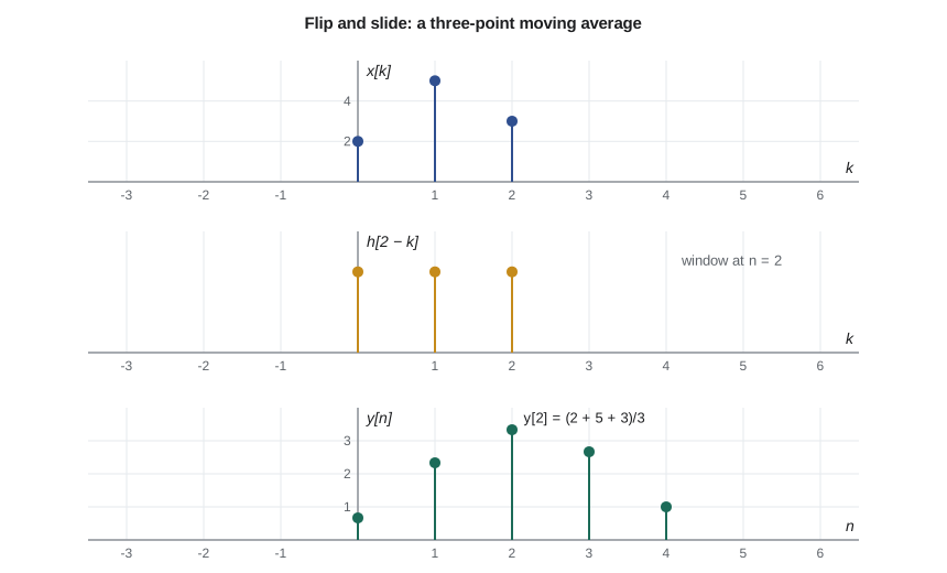
To compute one output value by hand, use the form y[n] = Σ x[k]h[n − k] and treat k as the running variable. First draw x[k]. Then draw h[−k], which is h flipped about k = 0. Sliding h[−k] to the right by n positions gives h[n − k]. Multiply the two sequences point by point and add the products; that sum is y[n]. Repeat for each n. For short sequences a table is faster: write x across the top, write h down the side, fill each cell with the product, and add along the diagonals.

Two general rules come out of the example. If x has length N and h has length M, the output has length N + M − 1. If x starts at index n₁ and h at n₂, the output starts at n₁ + n₂. These rules make a good check on hand calculations and on code.

Properties of convolution

Convolution behaves much like multiplication. It is commutative, x * h = h * x; associative, (x * h₁) * h₂ = x * (h₁ * h₂); and distributive over addition, x * (h₁ + h₂) = x * h₁ + x * h₂. The unit impulse is the identity, x * δ = x, and convolving with a shifted impulse shifts the signal, x[n] * δ[n − k] = x[n − k].

Each property has a system meaning. Associativity says two LTI systems in series act like one system whose impulse response is h₁ * h₂, and commutativity says their order does not matter. That is why Daniel can apply a moving average and then a scaling to convert to rpm, or scale first and average second, and get the same numbers apart from rounding. Distributivity says two systems in parallel act like one system with impulse response h₁ + h₂. The shift property says a pure delay of k samples has impulse response δ[n − k].

Reading system properties from h[n]

Because h[n] describes an LTI system completely, every property from lesson 2 can be read from it. The system is memoryless only if h[n] is zero except at n = 0, so that h[n] = Kδ[n]. It is causal if and only if h[n] = 0 for all n < 0, since a non-zero value at negative n would make the output respond before the impulse arrived. It is BIBO stable if and only if the impulse response is absolutely summable:

A finite impulse response (FIR) filter, such as any moving average, has only finitely many non-zero values, so it is always stable. An infinite impulse response (IIR) filter may or may not be. The filter with h[n] = aⁿu[n] is stable when |a| < 1, because the geometric series converges to 1/(1 − |a|), and unstable when |a| ≥ 1. The accumulator from lesson 2 has h[n] = u[n], which is the case a = 1, and the sum of |u[n]| diverges.

The step response

The response of an LTI system to the unit step, s[n], is the running sum of the impulse response, s[n] = Σ h[k] for k ≤ n, because u[n] is the running sum of δ[n]. The step response shows how a filter follows a sudden change, such as the pump being switched on. For the three-point average, s[n] climbs 1/3, 2/3, 1 and then stays at 1: the reading reaches its new value after three samples. A longer average smooths noise better but takes longer to respond, a trade-off that appears in every filter design.

import random
random.seed(7)

def conv(x, h):
    y = [0.0] * (len(x) + len(h) - 1)
    for k, xk in enumerate(x):           # each input sample launches a scaled copy of h
        for m, hm in enumerate(h):
            y[k + m] += xk * hm
    return y

print("hand example:", [round(v, 3) for v in conv([2, 5, 3], [1/3] * 3)])

# Tachometer: speed steps from 1200 to 1500 rpm at sample 10, plus noise
true = [1200] * 10 + [1500] * 20
meas = [v + random.gauss(0, 25) for v in true]
for M in (3, 8):
    y = conv(meas, [1 / M] * M)[:len(meas)]          # keep the causal part
    settled = next(n for n in range(10, 30) if abs(y[n] - 1500) < 30)
    noise = (sum((y[n] - 1500) ** 2 for n in range(20, 30)) / 10) ** 0.5
    print(f"{M}-point average: within 30 rpm at sample {settled}, rms error after = {noise:.1f} rpm")

raw = (sum((meas[n] - 1500) ** 2 for n in range(20, 30)) / 10) ** 0.5
print(f"raw readings: rms error = {raw:.1f} rpm")

hand example: [0.667, 2.333, 3.333, 2.667, 1.0]
3-point average: within 30 rpm at sample 12, rms error after = 11.4 rpm
8-point average: within 30 rpm at sample 17, rms error after = 8.9 rpm
raw readings: rms error = 19.6 rpm

The routine reproduces the hand result. On the simulated readings, the 8-point average is quieter than the 3-point average once it settles, but it needs more samples to reach the new speed after the step. The exact numbers depend on the random noise, but the pattern holds for any noise: averaging M readings of independent noise cuts its RMS value by about √M, while the delay to follow a step grows in proportion to M. Daniel chooses the length from the specification: the display must settle within about one second and must not wander by more than ±10 rpm.

Not every filter smooths

The same convolution sum describes filters that do the opposite of smoothing. The first difference, h[n] = δ[n] − δ[n − 1], gives y[n] = x[n] − x[n − 1], the change from one reading to the next. Its output is near zero while the pump runs steadily and spikes when the speed changes, so it acts as a change detector. Daniel uses it to flag sudden speed drops that can mean a clogged intake. A filter with h = [1, −2, 1] measures the change in the change, a discrete second derivative, and responds to bends in the speed curve. Smoothing filters have impulse responses whose values are all positive and add to one, so a steady input passes unchanged. Difference filters have values that add to zero, so a steady input gives zero output. Looking at the sum of h[n], which is the DC gain, tells you at a glance which kind of filter you have.

Convolution in firmware

On the microcontroller, the filter never sees a whole signal at once. Each time a new reading arrives, the firmware stores it in a circular buffer that holds the last M readings, overwriting the oldest one, and then computes y[n] = Σ h[k]x[n − k] over the buffer. This is the second form of the convolution sum, and it needs only M stored values and M multiplications per reading, however long the pump runs. The firmware also has to decide what the buffer holds before the first M readings arrive. Filling it with zeros reproduces the hand calculation above, with outputs that read low until the window is full; filling it with the first reading avoids that start-up dip. Both choices are common, and the specification should say which one is used.

Direct convolution costs N × M multiplications for N samples and an M-point filter. That is trivial for a moving average on a microcontroller, and a running-sum trick makes it cheaper still: add the new sample, subtract the one leaving the window. For long filters, lesson 10 shows how the fast Fourier transform does convolution far faster.