
ELE-250 · Lesson 2 of 12 · 24 min
Systems and their properties
A system transforms an input signal into an output signal. We write y(t) = T{x(t)} or, in discrete time, y[n] = T{x[n]}, where T is the rule that the system applies. The rule might be a circuit, a differential equation, a line of firmware or a physical process. At Cedarline, the systems in the pedestrian crossing controller include the microphone preamplifier from ELE-240, the anti-aliasing filter in front of the ADC, the averaging routine that smooths tachometer readings and the routine that turns measured street noise into a locator-tone volume. This lesson defines the properties that decide which mathematical tools apply to a system. The most important are linearity and time invariance, because systems that have both, called LTI systems, are completely described by a single response and can be analyzed with convolution and transforms.
Describing and connecting systems
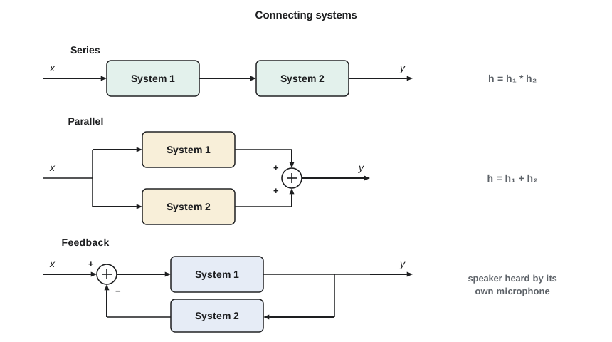
A block diagram draws each system as a box with an arrow in and an arrow out. Systems can be combined in three standard ways. In a series, or cascade, connection the output of the first system feeds the second; Amara's signal chain of preamplifier, filter and ADC is a cascade. In a parallel connection two systems receive the same input and their outputs are added, which is how a filter that keeps both low and high frequencies can be built. In a feedback connection the output is fed back and subtracted from the input; the automatic volume control on the locator tone is a feedback loop, because the speaker's own sound reaches the microphone and is measured as part of the noise.
Memory
A system is memoryless, or static, if its output at each time depends only on the input at that same time. A resistor, with v(t) = Ri(t), is memoryless, and so is an ideal amplifier with y(t) = 40x(t). A system with memory, or dynamic system, uses past or future input values. A capacitor, whose voltage is the integral of all past current, has memory, and so does a moving average, y[n] = (x[n] + x[n − 1] + x[n − 2] + x[n − 3])/4, which Cedarline uses to smooth the tachometer readings. Nearly every interesting system has memory, which is why most of this course is about how past inputs shape present outputs.
Causality
A system is causal if its output at any time depends only on present and past inputs, never on future ones. Every physical system that operates in real time is causal: the preamplifier cannot respond to sound that has not arrived yet. The moving average above is causal. The centred average y[n] = (x[n − 1] + x[n] + x[n + 1])/3 is not, because it needs x[n + 1]. Non-causal systems are still useful when the data are already recorded. If Daniel downloads a day of tachometer data to a laptop, he can smooth it with a centred average, which does not delay the features the way a causal average does. In real time, a non-causal filter can be made causal by delaying its output, which is exactly what happens when a centred average is computed one sample late.
Linearity
A system is linear if it satisfies superposition, which has two parts. Additivity means the response to x₁ + x₂ is the sum of the separate responses y₁ + y₂. Homogeneity, or scaling, means the response to a·x is a·y for any constant a. The two parts combine into one test:
A quick check catches many non-linear systems: a linear system must give zero output for zero input, because scaling the input by a = 0 must scale the output by zero. The system y(t) = 2x(t) + 3 fails that check, since zero input gives 3. It is called incrementally linear, meaning linear plus a constant offset, and the offset can be removed to leave a linear system. Squaring, rectifying, clipping and multiplying two signals together are non-linear. The microphone channel becomes non-linear when a passing bus is loud enough to drive the ADC to full scale and the samples are clipped, which is why Amara chose a preamplifier gain that leaves headroom.
Some systems that look complicated are linear. y(t) = t·x(t) is linear, because multiplying the input by a constant or adding two inputs passes straight through the multiplication by t. Linearity is about how the system treats its input, not about whether the formula contains time-varying coefficients.
Worked problem
Testing a system for linearity
Daniel proposes a noise estimator for the microphone: y[n] = x[n]², the instantaneous power. Is it linear?
Show solution
- Apply the test to a scaled input a·x[n].
- \[T\{a x[n]\} = \big(a x[n]\big)^2 = a^2 x[n]^2\]
- Compare with a times the original output.
- \[a\,T\{x[n]\} = a\,x[n]^2\]
- The two differ whenever a is not 0 or 1, so homogeneity fails.
Answer: The squarer is non-linear. That is not a flaw: measuring power is an inherently non-linear operation. It simply means the LTI tools in this course apply to the filters before and after the squarer, not to the squarer itself.
Time invariance
A system is time-invariant if a delay in the input causes the same delay in the output and nothing else. In symbols, if x(t) produces y(t), then x(t − t₀) must produce y(t − t₀) for every t₀. A circuit built from fixed resistors, capacitors and inductors is time-invariant: the same pulse gives the same response whether it arrives at noon or at midnight. The test is to compare two outputs. First delay the input and pass it through the system; then pass the original input through the system and delay the output. If the two results match for every input and delay, the system is time-invariant.
y(t) = t·x(t) fails this test. Delaying the input gives t·x(t − t₀), but delaying the output gives (t − t₀)·x(t − t₀), and those differ. The system is linear but time-varying, like a volume knob that someone turns slowly while a song plays. Downsampling, y[n] = x[2n], is also time-varying: delaying the input by one sample does not delay the output by one sample, and in fact it can change which samples survive. The locator tone's volume control is time-varying on purpose, because its gain follows the street noise.
Worked problem
Testing a system for time invariance
Is the system y(t) = x(2t), which plays a recording at double speed, time-invariant?
Show solution
- Delay the input by t₀ and then apply the system. Let v(t) = x(t − t₀); the system replaces t by 2t inside v.
- \[y_1(t) = v(2t) = x(2t - t_0)\]
- Now apply the system first and delay its output by t₀.
- \[y_2(t) = y(t - t_0) = x\big(2(t - t_0)\big) = x(2t - 2t_0)\]
- The two are different, because y₁ is shifted by t₀/2 while y₂ is shifted by t₀.
Answer: Time scaling is time-varying: a delay of t₀ in the input appears as a delay of only t₀/2 in the output. The system is still linear.
Stability
A system is bounded-input, bounded-output stable, or BIBO stable, if every bounded input produces a bounded output. If |x(t)| ≤ M for all t, the output must stay below some finite limit too. An amplifier with fixed gain is stable, and so is the moving average. An ideal integrator, y(t) = ∫x(τ)dτ, is not: a constant input, which is bounded, produces a ramp that grows without limit. Its discrete-time cousin, the accumulator y[n] = y[n − 1] + x[n], is unstable for the same reason. Stability matters in practice because a feedback loop that is unstable oscillates or saturates. If the locator tone's volume loop raises the volume whenever it hears the speaker, it can run away until the speaker is at full power; lessons 11 and 12 show how pole locations predict this.
Invertibility
A system is invertible if its input can be recovered exactly from its output, which requires that different inputs always give different outputs. y(t) = 5x(t) is invertible by y/5, and the accumulator is invertible by the first difference x[n] = y[n] − y[n − 1]. The squarer is not, because x and −x give the same output, and downsampling is not, because the discarded samples are gone. Equalizers in communication systems are designed as approximate inverses of the channel they follow.
| System | Memory | Causal | Linear | Time-invariant | BIBO stable |
|---|---|---|---|---|---|
| y(t) = 40x(t) | No | Yes | Yes | Yes | Yes |
| y[n] = (x[n] + … + x[n − 3])/4 | Yes | Yes | Yes | Yes | Yes |
| y[n] = x[n + 1] − x[n] | Yes | No | Yes | Yes | Yes |
| y(t) = ∫ x(τ) dτ from −∞ to t | Yes | Yes | Yes | Yes | No |
| y[n] = x[n]² | No | Yes | No | Yes | Yes |
| y(t) = t·x(t) | No | Yes | Yes | No | No |
| y(t) = 2x(t) + 3 | No | Yes | No (incrementally linear) | Yes | Yes |
Why LTI systems are special
A linear, time-invariant system is completely described by one function: its response to an impulse, written h(t) or h[n]. Because any input can be built from shifted, scaled impulses, linearity says the output is the same combination of shifted, scaled impulse responses, and time invariance says every shifted impulse gives the same shifted response. That combination is convolution, the subject of lessons 3 and 4.
LTI systems have a second, equally powerful property. A complex exponential input, e^(st) in continuous time or zⁿ in discrete time, comes out as the same exponential multiplied by a constant that depends on s or z:
Exponentials are therefore eigenfunctions of LTI systems, and H(s) or H(z) is the eigenvalue. With s = jω, a sinusoid of frequency ω comes out as a sinusoid of the same frequency, scaled in amplitude and shifted in phase by H(jω). That single fact is why filters can be described by frequency response, why the Fourier transform turns convolution into multiplication and why an LTI system can never create a frequency that was not in its input. When Amara sees a 120 Hz component at the output of a filter whose input contains only 60 Hz hum, she knows something in the chain is non-linear.
import math, random
random.seed(4)

def mavg(x):                      # 4-sample moving average, zero initial state
    return [sum(x[max(0, n - 3):n + 1]) / 4 for n in range(len(x))]
def square(x):
    return [v * v for v in x]
def ramp_gain(x):                 # y[n] = n * x[n]
    return [n * v for n, v in enumerate(x)]
def decimate(x):                  # y[n] = x[2n]
    return x[::2]

def delay(x, k):
    return [0.0] * k + x[:len(x) - k]

def close(a, b):
    return all(abs(p - q) < 1e-9 for p, q in zip(a, b))

N = 40
x1 = [random.uniform(-1, 1) for _ in range(N)]
x2 = [random.uniform(-1, 1) for _ in range(N)]
a, b = 2.5, -1.5
for name, T in (("moving average", mavg), ("squarer", square),
                ("n * x[n]", ramp_gain), ("decimate by 2", decimate)):
    lhs = T([a * p + b * q for p, q in zip(x1, x2)])
    rhs = [a * p + b * q for p, q in zip(T(x1), T(x2))]
    k = 2
    ti = close(T(delay(x1, k)), delay(T(x1), k))
print(f"{name:15s} linear: {str(close(lhs, rhs)):5s} time-invariant: {ti}")moving average linear: True time-invariant: True squarer linear: False time-invariant: True n * x[n] linear: True time-invariant: False decimate by 2 linear: True time-invariant: False
The moving average passes both tests, so it is LTI. The squarer is time-invariant but not linear, the n·x[n] system is linear but not time-invariant, and decimation is linear but fails the time-invariance test. Numerical tests like these are useful for checking firmware, but they are not proofs: a system could pass for the particular inputs tried and still fail for others. For a proof, use the algebraic tests in the worked examples.
Common mistakes
MistakeConcluding a system is linear because its formula has no squares.
InsteadCheck superposition directly; y(t) = 2x(t) + 3 has no squares but is not linear, and y(t) = t·x(t) is linear despite the t.
MistakeTesting time invariance by substituting t − t₀ everywhere, including in coefficients.
InsteadDelay only the input, apply the system, and compare with the delayed output.
MistakeAssuming every physical system must be stable.
InsteadAn integrator, an accumulator and many feedback loops are causal and physical but not BIBO stable.
MistakeCalling a non-causal filter useless.
InsteadNon-causal filters work on recorded data and can be made causal in real time by accepting a delay.
MistakeExpecting a linear filter to remove a frequency it cannot see, or to create a new one.
InsteadLTI systems only scale and shift the frequencies already present; new frequencies point to a non-linearity.
Summary and key terms
- Systems can be connected in series, parallel and feedback; block diagrams make the structure visible.
- Memoryless systems use only the present input; causal systems use only present and past inputs.
- A linear system obeys superposition: scaled sums in give the same scaled sums out, and zero in gives zero out.
- A time-invariant system responds to a delayed input with an equally delayed output.
- A BIBO-stable system turns every bounded input into a bounded output; integrators and accumulators are not BIBO stable.
- LTI systems are fully described by their impulse response, and complex exponentials pass through them scaled by H(s) or H(z).
- Causal system
- A system whose output depends only on present and past inputs.
- Linear system
- A system that satisfies additivity and homogeneity, so superposition holds.
- Time-invariant system
- A system for which a delay in the input produces the same delay in the output.
- BIBO stability
- The property that every bounded input produces a bounded output.
- LTI system
- A system that is both linear and time-invariant.
- Eigenfunction
- An input that passes through a system unchanged in form, only multiplied by a constant; complex exponentials for LTI systems.
- Incrementally linear
- Linear apart from a constant offset added to the output.
Practice problems
Work each problem on paper first, then reveal the answer to check.
Is y[n] = x[−n] causal? Is it time-invariant?
Show answer
Neither. For n < 0 it needs future inputs, and a delay in x becomes an advance in y.
Is y(t) = cos(x(t)) linear?
Show answer
No; cos(2x) ≠ 2cos(x), and zero input gives an output of 1.
Is y[n] = x[n] − 0.5x[n − 1] stable?
Show answer
Yes. If |x| ≤ M, then |y| ≤ 1.5M.
Is y(t) = x(t − 2) invertible? Give the inverse.
Show answer
Yes; x(t) = y(t + 2), an advance of 2.
Two LTI systems are in series. Can their order be swapped?
Show answer
Yes. The overall impulse response is the convolution of the two, and convolution is commutative.
Why can an LTI system not turn a 60 Hz input into 120 Hz?
Show answer
Complex exponentials are eigenfunctions, so each input frequency comes out at the same frequency, only scaled and shifted in phase.
Lesson quiz · 5 questions
Score 60% or more to complete this lesson.
Create a free account to save your progress, take quizzes and earn a certificate.