The discrete-time Fourier transform, the DFT and the FFT

Everything so far about spectra has used integrals over continuous time. The microcontroller in the pedestrian signal has none of that. It has blocks of samples, a few kilobytes of memory and a few milliseconds per block to decide how loud the street is and whether the locator tone is coming through clearly. This lesson gives the frequency-domain tools that work on samples. The discrete-time Fourier transform (DTFT) is the theory: the spectrum of an infinitely long sampled signal, and the frequency response of a digital filter. The discrete Fourier transform (DFT) is the practice: a finite sum over N samples that a computer can evaluate. The fast Fourier transform (FFT) is not a different transform but a clever algorithm that computes the DFT hundreds of times faster, and it is one of the most important algorithms in engineering.

The discrete-time Fourier transform

For a discrete-time signal x[n], the DTFT is

Ω is the discrete-time frequency in radians per sample. The DTFT is always periodic in Ω with period 2π, because e^(−j(Ω+2π)n) = e^(−jΩn) for every integer n; that is lesson 9's periodic spectrum seen from the discrete side. All the information lies in one period, usually −π to π. When x[n] comes from sampling at f_s, Ω connects to physical frequency by Ω = 2πf/f_s, so Ω = π corresponds to the Nyquist frequency f_s/2. At 8 kHz, the 880 Hz locator tone sits at Ω = 2π(880/8000) ≈ 0.691 rad per sample.

The DTFT has the same properties as the continuous transform. In particular, convolution becomes multiplication, so a digital filter's frequency response is the DTFT of its impulse response, H(e^(jΩ)) = Σh[n]e^(−jΩn). For an FIR filter this is a finite sum that can be evaluated directly.

From the DTFT to the DFT

The DTFT needs infinitely many samples and gives a function of a continuous variable, so a computer cannot evaluate it exactly. The DFT makes two compromises. It uses a block of N samples, x[0] to x[N − 1], and it evaluates the spectrum only at N equally spaced frequencies, Ω_k = 2πk/N:

Each X[k] is a complex number, and the index k is called a bin. Bin k corresponds to the physical frequency f_k = k·f_s/N, so the bin spacing, or frequency resolution, is Δf = f_s/N. A longer block gives finer resolution: at 8 kHz, a 256-sample block (32 ms) has bins 31.25 Hz apart, and a 1,024-sample block (128 ms) has bins 7.8 Hz apart. This is lesson 7's duration–bandwidth trade-off again: to resolve frequencies Δf apart, you must listen for at least 1/Δf seconds.

For real input, the bins above N/2 are mirror images of those below, X[N − k] = X[k]*, because they represent the negative frequencies. Bin 0 is the DC value times N, and bin N/2 is the Nyquist frequency. A single sinusoid of amplitude A that falls exactly on bin k gives |X[k]| = AN/2 and zero in every other bin below N/2, which is how a DFT-based meter converts bin values back to amplitudes.

Leakage and windows

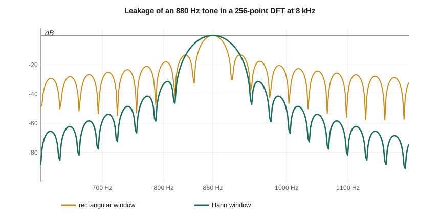
The DFT implicitly treats its N samples as one period of a periodic signal. If the block holds a whole number of cycles of a tone, the copies join smoothly and the tone falls in one bin. If not, the joins have a jump, and the jump's energy spreads into neighbouring bins. This spreading is spectral leakage. With 256 samples at 8 kHz, the 880 Hz tone falls at bin 880/31.25 = 28.16, between bins 28 and 29, so its energy leaks across many bins and its peak reads low. Leakage can hide a weak tone next to a strong one, which matters to Amara because she wants to measure a quiet locator tone in the presence of loud traffic.

There are two remedies. If the frequency of interest is known, choose N so that it falls on a bin: with N = 400 at 8 kHz, the bins are 20 Hz apart and 880 Hz is bin 44 exactly. If not, multiply the block by a window function that tapers smoothly to zero at both ends before taking the DFT. The Hann window, w[n] = ½(1 − cos(2πn/N)), is the usual choice. It makes each tone's peak a little wider but pushes the leaked energy far down, so weak tones become visible. Zero padding, appending zeros to a block before the DFT, gives more closely spaced bins that trace the spectrum more smoothly, but it adds no real resolution, because no new information about the signal has been added.

The fast Fourier transform

Evaluating the DFT directly takes N complex multiplications for each of N bins, N² in all: about 65,000 for N = 256 and a million for N = 1,024. The fast Fourier transform, popularized by Cooley and Tukey in 1965 though its core idea goes back to Gauss, cuts that to about (N/2)log₂N. For N a power of 2, the radix-2 FFT splits the samples into even- and odd-indexed halves, computes a half-length DFT of each, and combines them with one multiplication per pair, using the fact that the exponentials e^(−j2πkn/N) repeat. Applying the split recursively gives log₂N stages of N/2 operations. For N = 1,024 that is about 5,000 multiplications instead of a million, a speed-up of 200. On Cedarline's microcontroller, a 256-point FFT takes well under a millisecond, so the noise detector can update its spectrum every block.

Fast convolution

The FFT also makes long convolutions fast. Multiplying two DFTs and transforming back gives the circular convolution of the blocks, in which the end of the result wraps around to the beginning. Padding both sequences with zeros to at least N + M − 1 samples before the FFT prevents the wrap-around, so the result equals ordinary linear convolution. For a filter with hundreds of taps, transforming, multiplying and transforming back costs far less than direct convolution, and long signals are processed block by block with methods called overlap-add and overlap-save. Audio effects such as room reverberation, whose impulse responses last seconds, are run this way.

import cmath, math

def dft(x):
    N = len(x)
    return [sum(x[n] * cmath.exp(-2j * math.pi * k * n / N) for n in range(N)) for k in range(N)]

def fft(x):                                  # recursive radix-2, len(x) a power of 2
    N = len(x)
    if N == 1:
        return list(x)
    even, odd = fft(x[0::2]), fft(x[1::2])
    tw = [cmath.exp(-2j * math.pi * k / N) * odd[k] for k in range(N // 2)]
    return [even[k] + tw[k] for k in range(N // 2)] + [even[k] - tw[k] for k in range(N // 2)]

fs, N = 8000, 256
x = [math.cos(2 * math.pi * 880 * n / fs) for n in range(N)]
X1, X2 = dft(x), fft(x)
print("max |DFT - FFT| =", f"{max(abs(a - b) for a, b in zip(X1, X2)):.1e}")
print(f"multiplications: direct {N*N}, FFT about {N//2*int(math.log2(N))}")

def peak_and_far(x):
    X = fft(x)
    mag = [abs(v) for v in X[:N // 2]]
    top = max(mag)
    k = mag.index(top)
    far = max(mag[k + 8:k + 20])               # leakage 8 to 20 bins away
    return k, 20 * math.log10(far / top)

hann = [0.5 * (1 - math.cos(2 * math.pi * n / N)) for n in range(N)]
k, rect_db = peak_and_far(x)
_, hann_db = peak_and_far([a * w for a, w in zip(x, hann)])
print(f"peak in bin {k} ({k*fs/N:.1f} Hz); bin spacing {fs/N} Hz")
print(f"leakage 8-20 bins away: rectangular {rect_db:.0f} dB, Hann {hann_db:.0f} dB")

y = [math.cos(2 * math.pi * 880 * n / fs) for n in range(400)]
Y = dft(y)
print(f"N = 400: bin 44 magnitude {abs(Y[44]):.1f} (= N/2), bin 45 magnitude {abs(Y[45]):.1e}")

max |DFT - FFT| = 8.7e-12
multiplications: direct 65536, FFT about 1024
peak in bin 28 (875.0 Hz); bin spacing 31.25 Hz
leakage 8-20 bins away: rectangular -35 dB, Hann -70 dB
N = 400: bin 44 magnitude 200.0 (= N/2), bin 45 magnitude 5.2e-13

The DFT and FFT agree to rounding error, and the FFT needs about 1,000 multiplications instead of 65,536. The 880 Hz tone peaks in bin 28, at 875 Hz, the nearest bin. Without a window, the leakage 8 to 20 bins away is only about 35 dB below the peak; with the Hann window it drops to about 70 dB below, so a tone thousands of times weaker could be seen beside it. In the street, that difference decides whether the noise detector can still find the quiet locator tone while a loud truck passes on a nearby frequency. The cost of the window is a peak about twice as wide and a peak value about 6 dB lower, which the firmware corrects with a fixed scale factor, so Amara applies the Hann window to every block. With N = 400, the tone lands exactly in bin 44 with magnitude N/2 = 200 and essentially nothing in the next bin, as the theory says.