
CMPUT-474 · Lesson 11 of 12 · 32 min
Space complexity and the hierarchy theorems
Time is not the only resource that matters. Memory is often the tighter constraint, and space complexity has a surprisingly different character from time complexity. Space can be reused, while time cannot, which makes nondeterminism much less powerful for space than it appears to be for time: Savitch's theorem shows that nondeterministic space can be simulated deterministically with only a quadratic increase. This lesson defines the space classes, proves Savitch's theorem, introduces PSPACE and its complete problem TQBF, looks at logarithmic space and the classes L and NL, and then proves the hierarchy theorems, which show by diagonalization that more time or more space really does let us decide more languages. The hierarchy theorems give the few unconditional separations we know, such as \(\text{P} \ne \text{EXP}\).
Measuring space
The space used by a decider M on input w is the number of distinct tape cells it scans. Its space complexity \(s(n)\) is the maximum over inputs of length n, and \(\text{SPACE}(s(n))\) is the class of languages decided in \(O(s(n))\) space, with \(\text{NSPACE}(s(n))\) the nondeterministic version. For sublinear bounds such as \(\log n\), we use a machine with a read-only input tape and a separate work tape, and count only the work tape; otherwise even reading the input would cost linear space. Two basic relations connect time and space. A machine running in time t uses at most t cells, so \(\text{TIME}(t) \subseteq \text{SPACE}(t)\). Conversely, a machine using space \(s(n) \ge \log n\) has at most \(2^{O(s(n))}\) distinct configurations, and a decider never repeats a configuration, so \(\text{SPACE}(s) \subseteq \text{TIME}(2^{O(s)})\).
Space is generous. SAT is in linear space: try every assignment in turn, reusing the same cells for each. The same idea shows that all of NP lies in polynomial space, \(\text{NP} \subseteq \text{PSPACE}\), where \(\text{PSPACE} = \bigcup_k \text{SPACE}(n^k)\): to decide a language in NP, cycle through all certificates of polynomial length and run the verifier on each, erasing the work between attempts. The reuse of space across an exponential number of attempts is the characteristic move of space-bounded algorithms.
Savitch's theorem
Theorem (Savitch, 1970). For \(s(n) \ge \log n\), \(\text{NSPACE}(s(n)) \subseteq \text{SPACE}(s(n)^2)\). The proof is a clever reachability algorithm. A nondeterministic machine N using space s accepts w exactly when its configuration graph, with at most \(2^{O(s)}\) nodes, contains a path from the start configuration to an accepting one. Breadth-first search would find it but needs space for the visited set, which is exponential in s. Savitch's procedure \(\text{CANYIELD}(c_1, c_2, t)\) decides whether \(c_2\) is reachable from \(c_1\) in at most t steps by trying every possible midpoint m and recursively checking \(\text{CANYIELD}(c_1, m, t/2)\) and \(\text{CANYIELD}(m, c_2, t/2)\). Each recursive call reuses the same space after it returns.
The recursion depth is \(\log_2 t = O(s)\), because t starts at the number of configurations, \(2^{O(s)}\). Each level stores a constant number of configurations, each of size \(O(s)\). So the total space is \(O(s) \times O(s) = O(s^2)\). The running time is enormous, because the recursion tries every midpoint at every level, but space is what we are counting. The program below applies the procedure to reachability in a 64-vertex graph. The recursion depth stays at 4 for paths of length 8, while the number of calls runs into the hundreds of thousands: a vivid illustration of trading time for space.
# Savitch's theorem in miniature: decide reachability with a recursion that reuses space.
# CANYIELD(u, v, t): can v be reached from u in at most t steps? Try every midpoint m and
# recurse on both halves with t/2. Depth is log2(t); each level stores only (u, v, t, m).
import random
random.seed(474)
n = 64
edges = {u: set() for u in range(n)}
for u in range(n - 1):
    edges[u].add(u + 1) if random.random() < 0.9 else None
for _ in range(40):
    a, b = random.randrange(n), random.randrange(n)
    edges[a].add(b)

calls = 0; max_depth = 0
def can_yield(u, v, t, depth=1):
    global calls, max_depth
    calls += 1; max_depth = max(max_depth, depth)
    if t <= 1:
        return u == v or v in edges[u]
    h = (t + 1) // 2
    return any(can_yield(u, m, h, depth + 1) and can_yield(m, v, t - h, depth + 1) for m in range(n))

def bfs(u, v):
    seen, frontier = {u}, [u]
    while frontier:
        frontier = [w for x in frontier for w in edges[x] if w not in seen and not seen.add(w)]
    return v in seen, len(seen)

for (s, t) in [(0, 5), (0, 40), (17, 3)]:
    calls = 0; max_depth = 0
    r1 = can_yield(s, t, 8)
    r2, stored = bfs(s, t)
    print(f"{s:2d} -> {t:2d} within 8 steps: Savitch {r1!s:5} (recursion depth {max_depth}, {calls:7d} calls)   "
          f"BFS reachable at all: {r2!s:5} (stores {stored} vertices)")
print(f"Savitch stores O(log t) frames of O(log n) bits each; BFS stores up to n = {n} vertices.")
print("The price is time: the number of calls grows like n^(log t).")0 -> 5 within 8 steps: Savitch False (recursion depth 4, 287587 calls) BFS reachable at all: False (stores 59 vertices) 0 -> 40 within 8 steps: Savitch True (recursion depth 4, 101467 calls) BFS reachable at all: True (stores 59 vertices) 17 -> 3 within 8 steps: Savitch False (recursion depth 4, 327800 calls) BFS reachable at all: False (stores 57 vertices) Savitch stores O(log t) frames of O(log n) bits each; BFS stores up to n = 64 vertices. The price is time: the number of calls grows like n^(log t).
An immediate corollary is \(\text{NPSPACE} = \text{PSPACE}\): polynomial nondeterministic space squares to polynomial deterministic space. For time, the analogous question, whether \(\text{NP} = \text{P}\), is open. The difference is precisely reuse: a deterministic simulation of nondeterministic time has no evident way to avoid exploring exponentially many branches separately, while for space the recursion can explore them one after another in the same memory.
PSPACE-completeness and TQBF
A language is PSPACE-complete if it is in PSPACE and every language in PSPACE reduces to it in polynomial time. The canonical example is TQBF, the set of true fully quantified Boolean formulas, such as \(\forall x\, \exists y\, [(x \lor y) \land (\overline{x} \lor \overline{y})]\). TQBF is in PSPACE: evaluate the formula recursively, branching on the first quantified variable and combining the two results with 'or' for \(\exists\) and 'and' for \(\forall\); the recursion depth is the number of variables, and each level stores one bit. The program below does exactly this and shows that the order of quantifiers matters: swapping them in the example changes the answer, because a single y must then work for both values of x.
# TQBF: evaluating fully quantified Boolean formulas with polynomial space.
# Recursion on the quantifier prefix: space grows with the number of variables, not 2^n.
def evaluate(prefix, matrix, assign=None, depth=0, stats=None):
    assign = assign or {}; stats = stats if stats is not None else {"calls": 0, "depth": 0}
    stats["calls"] += 1; stats["depth"] = max(stats["depth"], depth)
    if not prefix:
        return all(any((l > 0) == assign[abs(l)] for l in c) for c in matrix), stats
    q, x = prefix[0]
    vals = (evaluate(prefix[1:], matrix, {**assign, x: b}, depth + 1, stats)[0] for b in (False, True))
    return (any(vals) if q == "E" else all(vals)), stats

# forall x1 exists x2 : (x1 or x2) and (not x1 or not x2)    -- x2 = not x1 works: TRUE
f1 = ([("A", 1), ("E", 2)], [(1, 2), (-1, -2)])
# exists x2 forall x1 : same matrix                          -- one x2 for both x1: FALSE
f2 = ([("E", 2), ("A", 1)], [(1, 2), (-1, -2)])
for name, (p, m) in (("forall x1 exists x2", f1), ("exists x2 forall x1", f2)):
    v, st = evaluate(p, m)
    print(f"{name}: {v}   ({st['calls']} calls, recursion depth {st['depth']})")
# a larger alternating formula over 16 variables: depth stays 16; short-circuiting keeps the
# number of calls below the 2^17 - 1 of a full search, but it still grows exponentially
prefix = [("A" if i % 2 else "E", i) for i in range(1, 17)]
matrix = [(i, -(i + 1)) for i in range(1, 16, 2)] + [(-i, i + 1) for i in range(1, 16, 2)]
v, st = evaluate(prefix, matrix)
print(f"16-variable formula: {v} ({st['calls']} calls, recursion depth {st['depth']})")forall x1 exists x2: True (6 calls, recursion depth 2) exists x2 forall x1: False (6 calls, recursion depth 2) 16-variable formula: True (3583 calls, recursion depth 16)
Theorem (Stockmeyer and Meyer, 1973). TQBF is PSPACE-complete. The hardness proof combines Cook–Levin with Savitch. For a machine M using polynomial space, write a formula \(\phi_{c_1, c_2, t}\) expressing 'configuration \(c_2\) is reachable from \(c_1\) in t steps'. Naively, \(\phi_{c_1,c_2,t} = \exists m\, [\phi_{c_1,m,t/2} \land \phi_{m,c_2,t/2}]\), but that doubles the formula size at each level, which would be exponential. The trick uses a universal quantifier to reuse one copy: \(\exists m\, \forall (c_3, c_4) \in \{(c_1, m), (m, c_2)\}\, [\phi_{c_3, c_4, t/2}]\). The size now grows by only a polynomial amount per level, and there are polynomially many levels. Many two-player games of perfect information have PSPACE-complete generalizations, because an alternation of 'there exists a move for me such that for all moves of my opponent' is exactly a quantifier alternation. Generalized geography is PSPACE-complete, and generalized chess and Go on n-by-n boards, with suitable rules, are PSPACE-hard or even EXPTIME-complete.
Logarithmic space: L and NL
The classes \(\text{L} = \text{SPACE}(\log n)\) and \(\text{NL} = \text{NSPACE}(\log n)\) capture computations that keep only a constant number of pointers into the input, since a pointer into an input of length n takes \(\log n\) bits. L contains arithmetic on numbers given in the input, checking balanced parentheses (keep a counter), and, by Reingold's 2005 theorem, undirected graph reachability. NL contains directed reachability, PATH: guess the path one vertex at a time, storing only the current vertex and a step counter. PATH is NL-complete under log-space reductions, which are reductions computable by log-space machines; polynomial-time reductions would be too strong, since everything in NL is in P. By Savitch, \(\text{NL} \subseteq \text{SPACE}(\log^2 n)\), and since a log-space machine has polynomially many configurations, \(\text{NL} \subseteq \text{P}\).
Theorem (Immerman and Szelepcsényi, 1987). \(\text{NL} = \text{coNL}\). Remarkably, a nondeterministic log-space machine can certify that a target vertex is not reachable, by an inductive counting technique: it computes the exact number of vertices reachable within i steps, for i = 0, 1, 2, and so on, using the count for i to verify the count for \(i + 1\), and finally checks that the target is not among the vertices reachable at all. The theorem, which earned both authors the 1995 Gödel Prize, contrasts with the widely believed \(\text{NP} \ne \text{coNP}\). Whether \(\text{L} = \text{NL}\) is open, as is whether \(\text{P} = \text{PSPACE}\).
The hierarchy theorems
Does more time let us decide more languages? Intuitively yes, but proving it requires diagonalization. A function \(t(n) \ge n \log n\) is time constructible if a machine can compute the binary representation of \(t(n)\) from \(1^n\) in time \(O(t(n))\); all the usual functions such as \(n^2\), \(n^k\) and \(2^n\) are. Time hierarchy theorem (Hartmanis and Stearns, 1965). For time-constructible t, there is a language decidable in \(O(t(n))\) time but not in \(o(t(n)/\log t(n))\) time. Space hierarchy theorem. For space-constructible \(s(n) \ge \log n\), there is a language decidable in \(O(s(n))\) space but not in \(o(s(n))\) space.
The proof builds a clocked diagonal machine D. On input \(\langle M \rangle\) of length n, D computes the budget \(t(n)\) and simulates M on \(\langle M \rangle\) for that many steps, counting as it goes. If M accepts within the budget, D rejects; if M rejects within the budget, D accepts; if the budget runs out, D rejects. D runs in \(O(t(n))\) time. Suppose some machine M decided L(D) in much less time. Then, on its own description, padded if necessary to make n large enough that the simulation overhead fits, M would finish within D's budget, and D would give the opposite answer, contradicting \(L(M) = L(D)\). The logarithmic gap in the time version pays for the overhead of simulating a machine with a different number of tapes and symbols; the space version has no gap because simulating space costs only a constant factor. The program below shows the clock in action on three toy machines.
# The idea behind the time hierarchy theorem: a clocked diagonal machine.
# D(<M>) simulates M on its own description for at most t(n) steps and flips the answer;
# if M has not finished, D rejects. Any machine running within the budget is contradicted.
# Here "machines" are Python generators; one yield = one step; the return value is the answer.
def m_fast(x):            # rejects after |x| steps
    for _ in x: yield
    return False
def m_quadratic(x):       # answers after |x|^2 steps
    for _ in range(len(x) ** 2): yield
    return True
def m_forever(x):
    while True: yield

def clocked(M, x, budget):
    g = M(x)
    for _ in range(budget):
        try: next(g)
        except StopIteration as e: return e.value
    return None

machines = {"m_fast": m_fast, "m_quadratic": m_quadratic, "m_forever": m_forever}
for name, M in machines.items():
    code = name * 10                      # stand-in for the machine's description
    n = len(code)
    for label, budget in (("t(n) = 7n", 7 * n), ("t(n) = n^3", n ** 3)):
        r = clocked(M, code, budget)
        d = "reject (budget exceeded)" if r is None else ("reject" if r else "accept")
print(f"{name:12s} n = {n:3d} {label:14s} M answers {str(r):5s} -> D says {d}")m_fast n = 60 t(n) = 7n M answers False -> D says accept m_fast n = 60 t(n) = n^3 M answers False -> D says accept m_quadratic n = 110 t(n) = 7n M answers None -> D says reject (budget exceeded) m_quadratic n = 110 t(n) = n^3 M answers True -> D says reject m_forever n = 90 t(n) = 7n M answers None -> D says reject (budget exceeded) m_forever n = 90 t(n) = n^3 M answers None -> D says reject (budget exceeded)
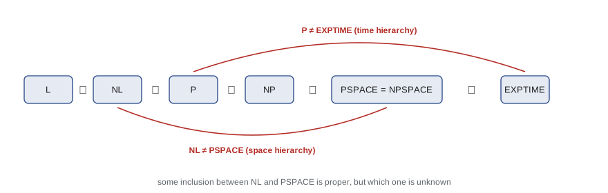
The theorems give the separations in the figure: \(\text{P} \subsetneq \text{EXPTIME}\), because \(n^k\) is \(o(2^n/n)\) for every k, and \(\text{NL} \subsetneq \text{PSPACE}\), because \(\log^2 n\) is \(o(n)\). Since \(\text{NL} \subseteq \text{P} \subseteq \text{NP} \subseteq \text{PSPACE}\), at least one of those inclusions must be proper, but which one is unknown. Concrete problems complete for EXPTIME, such as generalized chess under suitable rules, are therefore provably not in P, one of the few unconditional lower bounds for natural problems.
Why P versus NP is hard
If diagonalization separates P from EXPTIME, why not P from NP? In 1975 Baker, Gill and Solovay showed that there are oracles A and B with \(\text{P}^A = \text{NP}^A\) and \(\text{P}^B \ne \text{NP}^B\), where an oracle machine can ask membership questions about a fixed language in one step. Diagonalization arguments of the kind used above work equally well relative to any oracle, so no such argument alone can settle P versus NP, since it would have to give the same answer for A and B. This is the relativization barrier. Later work identified two more barriers, natural proofs (Razborov and Rudich, 1994), which limits a broad class of circuit lower-bound techniques if strong pseudorandom functions exist, and algebrization (Aaronson and Wigderson, 2008). Any proof that \(\text{P} \ne \text{NP}\) must use ideas that escape all three, which partly explains why the problem has resisted fifty years of effort.
| Class | Resource | Complete problem | Known relations |
|---|---|---|---|
| L | Deterministic log space | (under weaker reductions) undirected reachability | \(\text{L} \subseteq \text{NL}\) |
| NL | Nondeterministic log space | Directed reachability (PATH) | \(\text{NL} = \text{coNL} \subseteq \text{P}\) |
| P | Deterministic polynomial time | Circuit value (under log-space reductions) | \(\text{P} \subseteq \text{NP}\) |
| NP | Nondeterministic polynomial time | SAT, 3SAT, CLIQUE | \(\text{NP} \subseteq \text{PSPACE}\) |
| PSPACE | Polynomial space | TQBF, generalized geography | \(\text{PSPACE} = \text{NPSPACE}\) |
| EXPTIME | Exponential time | Generalized chess (suitable rules) | \(\text{P} \ne \text{EXPTIME}\) |
Worked examples
Worked problem
Space used by Savitch's algorithm
A nondeterministic machine uses 30 cells. How much space does the Savitch simulation need, roughly?
Show solution
- Configurations have size about 30 symbols plus state and head position, call it \(O(30)\).
- There are at most \(2^{O(30)}\) configurations, so the recursion depth is \(O(30)\).
- Each level stores a constant number of configurations.
- Total: \(O(30) \times O(30)\), on the order of a thousand cells.
Answer: Quadratic: on the order of \(30^2\) cells instead of 30.
Worked problem
Evaluating a QBF
Is \(\exists x\, \forall y\, (x \lor y) \land (x \lor \overline{y})\) true?
Show solution
- Try x = true: both clauses contain x, so they hold for every y.
- So there exists an x (namely true) such that for all y the matrix holds.
Answer: True.
Worked problem
Applying a hierarchy theorem
Is \(\text{TIME}(n^2) = \text{TIME}(n^3)\)?
Show solution
- \(n^3\) is time constructible.
- \(n^2 = o(n^3 / \log n^3)\), since \(n^3 / (3 \log n)\) grows faster than \(n^2\).
- By the time hierarchy theorem some language is in \(\text{TIME}(n^3)\) but not in \(\text{TIME}(n^2)\).
Answer: No; the inclusion is proper.
Common mistakes
MistakeAssume space and time behave the same under nondeterminism.
InsteadSavitch gives a quadratic simulation for space; for time no subexponential simulation is known.
MistakeCount the input tape when measuring logarithmic space.
InsteadUse a read-only input tape and count only the work tape.
MistakeUse polynomial-time reductions for NL-completeness.
InsteadThey are too strong; use log-space reductions.
MistakeWrite the reachability formula for TQBF hardness with two recursive copies.
InsteadThat doubles size each level; reuse one copy with a universal quantifier.
MistakeThink the hierarchy theorems separate P from NP.
InsteadThey separate classes with the same mode of computation and different bounds; P versus NP is blocked by relativization.
Summary and key terms
- Space counts cells used; \(\text{TIME}(t) \subseteq \text{SPACE}(t) \subseteq \text{TIME}(2^{O(t)})\).
- NP is contained in PSPACE, because certificates can be tried one at a time in reused space.
- Savitch: \(\text{NSPACE}(s) \subseteq \text{SPACE}(s^2)\), so NPSPACE = PSPACE.
- TQBF is PSPACE-complete; games with alternating moves often are too.
- L and NL use logarithmic work space; directed reachability is NL-complete, and NL = coNL.
- The time and space hierarchy theorems prove that more resources decide more languages, giving P ≠ EXPTIME and NL ≠ PSPACE.
- Relativization, natural proofs and algebrization are barriers to resolving P versus NP.
- Space complexity
- The maximum number of tape cells a decider scans on inputs of length n.
- PSPACE
- Languages decidable in polynomial space.
- Savitch's theorem
- Nondeterministic space s can be simulated in deterministic space s squared.
- TQBF
- The language of true fully quantified Boolean formulas, PSPACE-complete.
- L
- Languages decidable in logarithmic work space.
- NL
- Languages decidable in nondeterministic logarithmic space.
- Log-space reduction
- A reduction computable using logarithmic work space.
- Immerman-Szelepcsenyi theorem
- NL equals coNL.
- Time constructible
- A function whose value can be computed within that much time.
- Hierarchy theorem
- A result showing that more of a resource decides strictly more languages.
- Relativization
- The property that an argument works equally relative to any oracle.
Practice problems
Work each problem on paper first, then reveal the answer to check.
Why is SAT in linear space?
Show answer
Try every assignment in turn, reusing the same cells.
What is the recursion depth of CANYIELD for t steps?
Show answer
\(\log_2 t\).
What does Savitch give for NL?
Show answer
\(\text{NL} \subseteq \text{SPACE}(\log^2 n)\).
Name a PSPACE-complete problem.
Show answer
TQBF, or generalized geography.
Why is NL contained in P?
Show answer
A log-space machine has polynomially many configurations, so reachability in its configuration graph is polynomial.
Which classes do the hierarchy theorems separate?
Show answer
For example P from EXPTIME and NL from PSPACE.
What does the Baker-Gill-Solovay result show?
Show answer
Relativizing techniques cannot resolve P versus NP.
Is TIME(n) equal to TIME(n^2)?
Show answer
No, by the time hierarchy theorem.
Lesson quiz · 5 questions
Score 60% or more to complete this lesson.
Create a free account to save your progress, take quizzes and earn a certificate.