
CMPUT-411 · Lesson 1 of 12 · 34 min
Images, colour and compositing
Computer graphics is the science and craft of making pictures with computers: turning a description of a scene, such as geometry, materials, lights and a camera, into an image that a person sees on a display. It underlies video games and film visual effects, computer-aided design, scientific and medical visualization, maps, user interfaces, and increasingly the synthetic data used to train vision systems. This course follows the path from numbers to pixels. It starts with what an image is and how colour is represented, moves through rasterization, transformations, cameras and the hardware pipeline of a graphics processing unit (GPU), and ends with ray tracing, path tracing and the neural methods that have joined the field in the last few years.
Throughout the course we build a small software renderer in Python, a few hundred lines in total, so that each idea becomes something you can run and inspect. Real renderers run on GPUs and are written in C++, shading languages and GPU APIs, but the mathematics is the same, and seeing it in a few lines of plain code is the fastest way to understand what the hardware is doing. The prerequisites are data structures and algorithms (CMPUT-204) and linear algebra (MATH-125); we use vectors, matrices, dot and cross products and linear transformations constantly.
Raster images and framebuffers
A raster image is a rectangular grid of picture elements, or pixels, each storing a colour. A 1920 by 1080 image has about 2.07 million pixels; a 3840 by 2160 (4K) image has about 8.3 million. The memory that holds the image being displayed is the framebuffer. A display refreshes from it at a fixed rate, commonly 60 to 144 times per second, and renderers usually draw into a back buffer while the front buffer is shown, then swap them (double buffering) so the viewer never sees a half-drawn frame. Synchronizing the swap with the display's refresh (vertical sync) avoids tearing, at the cost of waiting; variable refresh rate displays adapt the refresh to the renderer instead.
It is tempting to think of a pixel as a little square, but in signal processing terms a pixel is a sample of a continuous image at a point, and the display reconstructs a continuous picture from those samples. Alvy Ray Smith's 1995 memo 'A pixel is not a little square' made this argument forcefully. The distinction matters for antialiasing (lesson 2) and texture filtering (lesson 9): treating pixels as point samples explains why sampling too coarsely produces aliasing and why good filters weight neighbouring samples smoothly.
Each pixel typically stores red, green and blue (RGB) components, because human colour vision has three types of cone cells and three primaries can reproduce a large range of colours. In the common 8-bit-per-channel format, each component is an integer from 0 to 255, giving about 16.7 million combinations. High dynamic range (HDR) rendering stores components as floating-point numbers, usually 16-bit half floats, so that values brighter than display white (the sun, a specular highlight) can be represented and later compressed to the display's range by tone mapping. A fourth channel, alpha, often stores coverage or opacity, which we use for compositing below.
| Format | Bits per pixel | Typical use |
|---|---|---|
| 8-bit grey | 8 | Masks, single-channel data such as height maps |
| RGBA8 (sRGB-encoded) | 32 | Display images, textures for colour |
| RGBA16F (half float, linear) | 64 | HDR rendering targets before tone mapping |
| RGBA32F (float, linear) | 128 | Accumulation buffers, offline rendering, scientific images |
| Depth 24 + stencil 8 | 32 | Depth buffer (lesson 6) and stencil masks |
| BC1 to BC7, ASTC (compressed) | 4 to 8 | GPU texture compression for colour and normal maps |
Light, colour and the eye
Colour is a perception, not a physical property of light alone. Light is electromagnetic radiation, and visible light spans wavelengths of roughly 380 to 750 nanometres. A light source or surface has a spectral power distribution, the amount of power at each wavelength. The retina has three kinds of cone cells, called S, M and L for short, medium and long wavelengths, each with a broad sensitivity curve. The brain receives only three numbers per point, the responses of the three cone types, so many different spectra produce identical cone responses and therefore the same perceived colour. Such spectra are called metamers, and metamerism is what makes three-primary displays possible: a monitor does not reproduce the spectrum of a lemon, only a spectrum that excites the cones the same way.
In 1931 the Commission internationale de l'éclairage (CIE) standardized colour matching functions and the XYZ colour space, in which any visible colour has non-negative coordinates and Y corresponds to luminance, the perceived brightness of light. Display colour spaces such as sRGB are defined relative to XYZ by the chromaticities of their red, green and blue primaries and a white point. sRGB, standardized in 1996 for monitors and the web, uses the same primaries as the HDTV standard BT.709 and the D65 white point, which approximates average daylight. Its gamut, the set of colours it can show, is a triangle within the horseshoe of visible chromaticities; wider gamuts such as Display P3 (used by many phones and laptops) and BT.2020 (for HDR video) cover more of it. PHOT-301 treats colour science and ICC colour management in depth for photographers; here we need the parts that matter for rendering.
RGB spaces are convenient for hardware but poor for describing colours to people and for measuring differences. Hue, saturation and value (HSV) and hue, saturation and lightness (HSL) rearrange RGB into cylinder coordinates that match how designers pick colours: hue as an angle around a colour wheel, saturation as distance from grey, value or lightness as height. They are simple transformations of RGB, not perceptual spaces. CIELAB (1976) is designed to be approximately perceptually uniform: L* measures lightness from 0 (black) to 100 (white), a* runs from green to red and b* from blue to yellow, and the Euclidean distance between two colours, \(\Delta E^*_{ab}\), approximates how different they look, with a difference of about 2.3 near the threshold of noticing. Later formulas such as CIEDE2000 correct remaining non-uniformities, and newer spaces such as Oklab (2020) are popular in graphics for smooth gradients.
# From sRGB to CIE XYZ and CIELAB, and a perceptual difference (Delta E 1976)
# between two shades that look similar in RGB terms but not to the eye.
M = [[0.4124, 0.3576, 0.1805],      # linear sRGB (D65) to XYZ
     [0.2126, 0.7152, 0.0722],
     [0.0193, 0.1192, 0.9505]]
WHITE = (0.95047, 1.0, 1.08883)     # D65 reference white
def lin(c): return c / 12.92 if c <= 0.04045 else ((c + 0.055) / 1.055) ** 2.4
def xyz(rgb8):
    r, g, b = (lin(v / 255) for v in rgb8)
    return tuple(m[0] * r + m[1] * g + m[2] * b for m in M)
def lab(rgb8):
    def f(t): return t ** (1 / 3) if t > (6 / 29) ** 3 else t / (3 * (6 / 29) ** 2) + 4 / 29
    fx, fy, fz = (f(v / w) for v, w in zip(xyz(rgb8), WHITE))
    return (116 * fy - 16, 500 * (fx - fy), 200 * (fy - fz))
def dE(a, b): return sum((x - y) ** 2 for x, y in zip(lab(a), lab(b))) ** 0.5
pairs = [((0, 0, 255), (0, 0, 205)),      # two blues 50 codes apart
         ((0, 255, 0), (0, 205, 0)),      # two greens 50 codes apart
         ((128, 128, 128), (138, 128, 128))]
for p, r in pairs:
    L1, a1, b1 = lab(p)
    print(f"{p} vs {r}: Lab of first = ({L1:.1f}, {a1:.1f}, {b1:.1f}), Delta E = {dE(p, r):.1f}")
print("relative luminance Y of pure R, G, B:", [round(xyz(c)[1], 4) for c in ((255, 0, 0), (0, 255, 0), (0, 0, 255))])(0, 0, 255) vs (0, 0, 205): Lab of first = (32.3, 79.2, -107.9), Delta E = 21.6 (0, 255, 0) vs (0, 205, 0): Lab of first = (87.7, -86.2, 83.2), Delta E = 24.0 (128, 128, 128) vs (138, 128, 128): Lab of first = (53.6, 0.0, -0.0), Delta E = 4.1 relative luminance Y of pure R, G, B: [0.2126, 0.7152, 0.0722]
The output illustrates two facts that recur throughout graphics. Equal steps in RGB codes are not equal perceptual steps: the two blues 50 codes apart differ by a smaller \(\Delta E\) than the two greens 50 codes apart, and a 10-code change in a grey's red channel produces a modest difference. And the three primaries contribute very unequally to luminance: green supplies about 72 per cent of the luminance of white, red about 21 per cent and blue only about 7 per cent. That is why converting colour images to grey with equal weights looks wrong, and why the relative luminance used in accessibility contrast checks weights the channels \(0.2126 R + 0.7152 G + 0.0722 B\) in linear light.
Gamma and the sRGB transfer function
Pixel values in ordinary images are not proportional to light. Human lightness perception is roughly logarithmic or power-law: we distinguish dark shades much more finely than bright ones. If 8-bit codes were spread evenly in light intensity, most codes would be wasted on bright values we cannot tell apart, and the darks would show visible banding. So images are encoded with a nonlinear transfer function that spends more codes on darks. Historically this matched the response of cathode-ray tubes, whose light output was roughly the input voltage raised to a power of about 2.2, called gamma. The sRGB standard defines a transfer function that is linear near black and a power of 2.4 with an offset elsewhere, which overall approximates a gamma of 2.2.
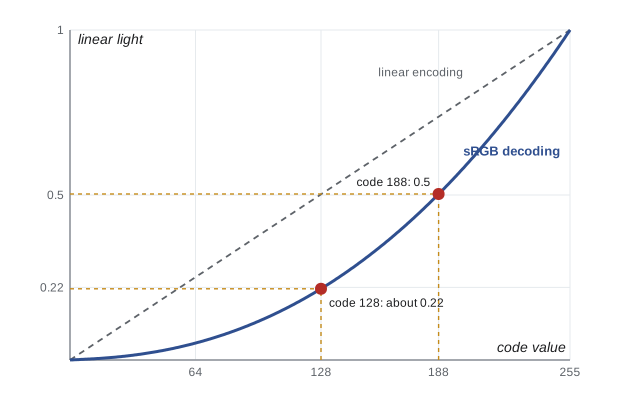
The practical rule is simple and is violated surprisingly often: do arithmetic on light in linear space, and encode to sRGB only for storage and display. Lighting calculations add and scale light, blending averages it, and filtering and antialiasing average neighbouring samples; all of these are physically meaningful only on values proportional to light. Doing them on sRGB-encoded values makes antialiased edges look too dark and thin, mixes of colours look muddy, and lighting falls off unnaturally. GPUs help: a texture or render target declared with an sRGB format is decoded to linear automatically when sampled and encoded automatically when written, so shaders work in linear space without explicit conversions.
# sRGB transfer functions, why averaging must happen in linear light, and the
# Porter-Duff "over" operator with straight and premultiplied alpha.
def to_linear(c):            # c in [0, 1], an sRGB-encoded value
    return c / 12.92 if c <= 0.04045 else ((c + 0.055) / 1.055) ** 2.4
def to_srgb(x):              # x in [0, 1], linear light
    return 12.92 * x if x <= 0.0031308 else 1.055 * x ** (1 / 2.4) - 0.055
def q8(c): return round(255 * c)
for code in (0, 64, 128, 188, 255):
    print(f"sRGB code {code:3} -> linear {to_linear(code / 255):.4f}")
# A 50% coverage edge pixel between black and white
naive = (0 + 1) / 2                                  # averaging encoded values
right = to_srgb((to_linear(0) + to_linear(1)) / 2)   # averaging light, then encoding
print(f"edge pixel: naive average code {q8(naive)}, linear-light average code {q8(right)}")
# Porter-Duff over: source (front) over destination (back), per channel
def over_straight(cs, a_s, cd, a_d):
    a_o = a_s + a_d * (1 - a_s)
    c_o = (cs * a_s + cd * a_d * (1 - a_s)) / a_o if a_o > 0 else 0.0
    return c_o, a_o
def over_premul(ps, a_s, pd, a_d):                   # p = c * alpha already
    return ps + pd * (1 - a_s), a_s + a_d * (1 - a_s)
front = (0.9, 0.4)            # linear red channel 0.9 with alpha 0.4
back = (0.2, 1.0)             # opaque background, red 0.2
print("straight over:", tuple(round(v, 4) for v in over_straight(front[0], front[1], back[0], back[1])))
p = over_premul(front[0] * front[1], front[1], back[0] * back[1], back[1])
print("premultiplied over:", tuple(round(v, 4) for v in p), "-> straight", round(p[0] / p[1], 4))
# Downsampling a half-transparent red pixel next to an opaque blue one (red, blue, alpha)
a = (1.0, 0.0, 0.0, 0.0); b = (0.0, 0.0, 1.0, 1.0)  # fully transparent "red" and opaque blue
straight = tuple((x + y) / 2 for x, y in zip(a, b))
pa = (a[0] * a[3], a[1] * a[3], a[2] * a[3], a[3]); pb = (b[0] * b[3], b[1] * b[3], b[2] * b[3], b[3])
pm = tuple((x + y) / 2 for x, y in zip(pa, pb))
print("filter straight:", straight, " filter premultiplied:", pm)sRGB code 0 -> linear 0.0000 sRGB code 64 -> linear 0.0513 sRGB code 128 -> linear 0.2159 sRGB code 188 -> linear 0.5029 sRGB code 255 -> linear 1.0000 edge pixel: naive average code 128, linear-light average code 188 straight over: (0.48, 1.0) premultiplied over: (0.48, 1.0) -> straight 0.48 filter straight: (0.5, 0.0, 0.5, 0.5) filter premultiplied: (0.0, 0.0, 0.5, 0.5)
The first lines show the nonlinearity: code 128 is about 22 per cent of full light, while code 188 is about half. The edge pixel half covered by a white shape on black should emit half the light of white, which is code 188 when encoded; naive averaging of encoded values gives 128, which is too dark, and is why gamma-incorrect antialiasing makes text and lines look thin and jagged.
Alpha and compositing
Compositing combines images in layers: a rendered character over a painted background, a user interface over a game scene, a visual effects element over live-action footage. Thomas Porter and Tom Duff's 1984 paper 'Compositing digital images' introduced the alpha channel as a standard part of an image and defined an algebra of twelve compositing operators. Alpha \(\alpha\) represents the fraction of a pixel covered by the element, or its opacity, from 0 (fully transparent) to 1 (fully opaque). The most important operator is over, which places a source element A in front of a destination B.
With straight (unassociated) alpha, colours are stored independently of alpha, and every compositing step multiplies by alpha and divides again. With premultiplied (associated) alpha, each stored colour is already multiplied by its alpha, so the pixel stores \((C\alpha, \alpha)\). The over operator becomes a single multiply-add per channel, \(P_o = P_A + P_B(1 - \alpha_A)\), the same formula for colour and alpha. Premultiplied alpha has a more important advantage than speed: it makes filtering correct. When an image is blurred, downsampled or interpolated, neighbouring pixels are averaged. With straight alpha, a fully transparent pixel's arbitrary colour leaks into the result; the program's last line shows a transparent 'red' pixel averaged with an opaque blue one producing a half-transparent purple, a dark or coloured fringe familiar from badly made textures. With premultiplied alpha, the transparent pixel contributes nothing, and the result is half-transparent pure blue, as it should be. For this reason GPU blending, texture filtering and most compositing systems prefer premultiplied alpha.
GPUs implement compositing in fixed-function blending hardware. The blend equation combines the fragment being written (source) with the value already in the framebuffer (destination) using configurable factors; premultiplied over uses a source factor of one and a destination factor of one minus source alpha. Because over is not commutative, transparent surfaces must be drawn in back-to-front order, which is one of the persistent headaches of real-time rendering; order-independent transparency techniques, such as depth peeling and weighted blended transparency, approximate the result without sorting.
Displays, bit depth and HDR
Displays convert encoded values to light with their own characteristics, and colour-managed systems use profiles to map between the image's colour space and the display's. Standard dynamic range displays reach roughly 100 to 300 candelas per square metre (nits) and are assumed to show sRGB. HDR displays reach 1,000 nits or more and use different transfer functions designed for wide brightness ranges, such as the perceptual quantizer (PQ, SMPTE ST 2084) and hybrid log-gamma (HLG). With only 8 bits, smooth gradients such as skies can show banding, especially after processing; rendering in floating point and adding a small amount of noise before quantization, called dithering, breaks up bands so the eye averages them away.
Rendering engines therefore work in a scene-referred linear space with floating-point values, apply exposure and tone mapping to compress the scene's range into the display's, and then apply the display's transfer function. Tone mapping operators range from the simple Reinhard curve \(L/(1+L)\) to the filmic curves used in games and the Academy Color Encoding System (ACES) used in film. Getting this chain right, linear lighting, correct transfer functions and sensible tone mapping, is the single most effective improvement many beginners can make to their renders.
Worked examples
Worked problem
Decoding sRGB
What fraction of full light does an sRGB code value of 64 represent?
Show solution
- Normalize: \(64/255 = 0.2510\). This is above 0.04045, so use the power branch.
- \(((0.2510 + 0.055)/1.055)^{2.4} = (0.2900)^{2.4}\).
- \(\ln 0.2900 = -1.2379\); times 2.4 gives \(-2.971\); \(e^{-2.971} = 0.0513\).
Answer: About 0.051, or 5 per cent of full light, even though 64 is a quarter of the code range.
Worked problem
Compositing with premultiplied alpha
A premultiplied source pixel (0.36, 0.10, 0.05, alpha 0.4) is composited over an opaque destination (0.20, 0.30, 0.60, alpha 1). Find the result.
Show solution
- Each channel: \(P_o = P_A + P_B(1 - \alpha_A) = P_A + 0.6 P_B\).
- Red \(0.36 + 0.6 \times 0.20 = 0.48\); green \(0.10 + 0.18 = 0.28\); blue \(0.05 + 0.36 = 0.41\).
- Alpha \(0.4 + 0.6 \times 1 = 1.0\).
Answer: (0.48, 0.28, 0.41, 1.0); because the result is opaque, these premultiplied values are also the straight colour.
Worked problem
Memory for a framebuffer
How much memory do a 3840 by 2160 RGBA16F colour target and a 32-bit depth buffer need?
Show solution
- Pixels: \(3840 \times 2160 = 8{,}294{,}400\).
- Colour: 8 bytes per pixel, so 66.4 MB. Depth: 4 bytes per pixel, so 33.2 MB.
- Total about 99.5 MB, before double buffering or any additional render targets.
Answer: About 100 MB, which is why modern renderers budget GPU memory for render targets carefully.
Common mistakes
MistakeAverage or blend sRGB-encoded pixel values directly.
InsteadDecode to linear light, do the arithmetic, then encode; or use sRGB texture and render-target formats that do this automatically.
MistakeAssume equal RGB steps are equal perceptual steps.
InsteadUse a perceptual space such as CIELAB or Oklab to measure or interpolate colour differences.
MistakeStore straight alpha and filter or downsample the image.
InsteadUse premultiplied alpha so transparent pixels contribute nothing to filtered results.
MistakeTreat a pixel as a small solid square.
InsteadTreat pixels as point samples of a continuous image; this explains aliasing and guides filtering.
MistakeClamp lighting results to 1.0 at every step.
InsteadRender in floating point and tone map at the end so bright values keep their relationships.
Summary and key terms
- A raster image is a grid of pixel samples held in a framebuffer and shown by a display at a fixed refresh rate.
- Three cone types make colour three-dimensional, so three primaries can reproduce many colours through metamerism.
- CIE XYZ is the reference colour space; sRGB, Display P3 and BT.2020 are defined by primaries and a white point.
- CIELAB approximates perceptual uniformity, and Euclidean distances in it estimate visible differences.
- The sRGB transfer function spends more codes on darks; code 128 is only about 22 per cent of full light.
- Lighting, blending and filtering must be done in linear light, with encoding only for storage and display.
- Premultiplied alpha makes the over operator a single multiply-add and makes filtering correct.
- Pixel
- A sample of an image at one location, storing a colour and often an alpha value.
- Framebuffer
- The memory holding the image that is displayed or being rendered.
- Metamers
- Different light spectra that produce the same cone responses and so look identical.
- Gamut
- The set of colours a device or colour space can represent.
- Transfer function
- The nonlinear mapping between encoded values and linear light, such as the sRGB curve.
- Linear light
- Pixel values proportional to physical light intensity.
- CIELAB
- A colour space designed so that distances approximate perceived colour differences.
- Alpha
- A per-pixel value giving coverage or opacity, from 0 to 1.
- Premultiplied alpha
- A representation in which colour channels are stored already multiplied by alpha.
- Tone mapping
- Compressing a high dynamic range of scene values into the range a display can show.
Practice problems
Work each problem on paper first, then reveal the answer to check.
How many pixels does a 2560 by 1440 image contain?
Show answer
About 3.69 million.
Why can a display with three primaries reproduce the appearance of a lemon?
Show answer
Because of metamerism: it only needs to produce the same cone responses, not the same spectrum.
Which primary contributes most to luminance in sRGB?
Show answer
Green, about 72 per cent of white's luminance.
What linear light value corresponds to sRGB code 255?
Show answer
1.0, full light.
Why does naive averaging of sRGB values make antialiased edges look thin?
Show answer
Averaged codes encode less light than the true average, so edge pixels are too dark.
Write the over operator for premultiplied alpha.
Show answer
\(P_o = P_A + P_B(1-\alpha_A)\), applied to colour and alpha alike.
Why must transparent surfaces usually be sorted back to front?
Show answer
The over operator is not commutative.
What does a CIELAB difference of about 2.3 signify?
Show answer
Roughly a just noticeable difference.
What is dithering used for?
Show answer
Adding small noise before quantization to hide banding in smooth gradients.
Name two HDR transfer functions.
Show answer
PQ (SMPTE ST 2084) and HLG.
Lesson quiz · 5 questions
Score 60% or more to complete this lesson.
Create a free account to save your progress, take quizzes and earn a certificate.