The lambda calculus

In 1936, before there were any electronic computers, Alonzo Church published a tiny formal system for describing functions. It has just three constructs: variables, function definitions and function applications. Church's lambda calculus turned out to be as powerful as Alan Turing's machines, which Turing showed the same year, and it became the theoretical core of functional programming. Lisp, ML, Haskell and the lambda expressions in Python, Java, C# and C++ all descend from it. This lesson defines the calculus, implements its reduction rules carefully, shows how numbers and data can be built from functions alone, and explains how recursion works without names.

Lesson 4 gave us the vocabulary of free and bound variables, environments and closures. The lambda calculus strips all of that down to substitution, which is why it is the standard testing ground for ideas about evaluation (lesson 6) and types (lessons 7 and 8). CMPUT-474 proves that the calculus is Turing-complete and that some questions about its terms, such as whether a term has a normal form, cannot be decided.

Syntax

A lambda term is one of three things: a variable such as x; an abstraction λx.M, the function with parameter x and body M; or an application M N, the function M applied to the argument N. Two conventions keep terms readable. Application associates to the left, so f a b means (f a) b. The body of an abstraction extends as far to the right as possible, so λx.f x y means λx.((f x) y). We also abbreviate λx.λy.M as λx y.M. There are no numbers, no Booleans, no let and no recursion built in; we will build all of them.

Alpha conversion, substitution and beta reduction

Alpha conversion says that the names of bound variables do not matter: λx.x and λy.y are the same function. Terms that differ only in bound names are alpha-equivalent. Beta reduction is the computation rule: applying a function to an argument substitutes the argument for the parameter in the body.

The subtle part is substitution. Substituting naively can capture a free variable, changing the meaning of a term. Consider (λx.λy.x) y. The function returns its first argument, so applied to the free variable y it should give a function that ignores its argument and returns that outer y. Naive substitution would produce λy.y, the identity function, because the outer y has been captured by the inner binder. Capture-avoiding substitution first renames the inner bound variable to something fresh, giving λv0.y, which is correct. Getting this right is the first bug every implementer of a functional language has to fix.

# A complete untyped lambda calculus: parser, printer, capture-avoiding substitution
# and a normal-order reducer.  Terms: ("var", x) | ("lam", x, body) | ("app", f, a)
import re, itertools

def parse(src):
    toks = re.findall(r"\\|\.|\(|\)|[A-Za-z_][A-Za-z_0-9']*", src); pos = 0
    def peek(): return toks[pos] if pos < len(toks) else None
    def eat(t=None):
        nonlocal pos
        tok = toks[pos]; assert t is None or tok == t, (t, tok); pos += 1; return tok
    def term():
        if peek() == "\\":
            eat("\\"); params = []
            while peek() != ".": params.append(eat())
            eat("."); body = term()
            for p in reversed(params): body = ("lam", p, body)
            return body
        f = atom()
        while peek() not in (None, ")"):
            f = ("app", f, atom() if peek() != "\\" else term())   # application is left-associative
        return f
    def atom():
        if peek() == "(":
            eat("("); t = term(); eat(")"); return t
        return ("var", eat())
    return term()

def show(t):
    if t[0] == "var": return t[1]
    if t[0] == "lam": return "\u03bb" + t[1] + "." + show(t[2])
    f = show(t[1]) if t[1][0] != "lam" else "(" + show(t[1]) + ")"
    a = show(t[2]) if t[2][0] == "var" else "(" + show(t[2]) + ")"
    return f + " " + a

def free(t):
    if t[0] == "var": return {t[1]}
    if t[0] == "lam": return free(t[2]) - {t[1]}
    return free(t[1]) | free(t[2])

fresh_names = (f"v{i}" for i in itertools.count())
def subst(t, x, s):
    """t[x := s], renaming bound variables to avoid capture."""
    if t[0] == "var": return s if t[1] == x else t
    if t[0] == "app": return ("app", subst(t[1], x, s), subst(t[2], x, s))
    y, body = t[1], t[2]
    if y == x: return t                                  # x is shadowed: stop
    if y in free(s):                                     # would capture: alpha-rename y first
        z = next(fresh_names); body = subst(body, y, ("var", z)); y = z
    return ("lam", y, subst(body, x, s))

def step(t):
    """One normal-order step (leftmost-outermost redex first), or None if t is in normal form."""
    if t[0] == "app":
        if t[1][0] == "lam":
            return subst(t[1][2], t[1][1], t[2])         # beta reduction
        r = step(t[1])
        if r is not None: return ("app", r, t[2])
        r = step(t[2])
        if r is not None: return ("app", t[1], r)
    if t[0] == "lam":
        r = step(t[2])
        if r is not None: return ("lam", t[1], r)
    return None

def normalize(src, trace=True, limit=100):
    t = parse(src); n = 0
    while True:
        if trace: print(f"  {n:2}: {show(t)}")
        nxt = step(t)
        if nxt is None: return t, n
        t, n = nxt, n + 1
        if n > limit: raise RuntimeError("no normal form within the step limit")

print("(\u03bbx.\u03bby.x) a b")
normalize(r"(\x y. x) a b")
print("capture-avoiding substitution: (\u03bbx.\u03bby.x y) y")
normalize(r"(\x. \y. x y) y")

(λx.λy.x) a b
   0: (λx.λy.x) a b
   1: (λy.a) b
   2: a
capture-avoiding substitution: (λx.λy.x y) y
   0: (λx.λy.x y) y
   1: λv0.y v0

A third rule, eta conversion, says λx.M x is equivalent to M when x is not free in M: both behave the same when applied to any argument. Compilers use eta conversion when they simplify wrappers such as lambda x: f(x) into plain f.

Normal forms and evaluation order

A term with no beta redex (no application of a lambda to an argument) is in normal form, and normal forms play the role of final answers. Some terms have no normal form. The classic example is Ω = (λx.x x)(λx.x x), which reduces to itself forever. When a term contains several redexes, the order in which we reduce them matters. Normal order always reduces the leftmost, outermost redex first. Applicative order reduces the arguments of an application before the application itself, which is how most programming languages evaluate function calls.

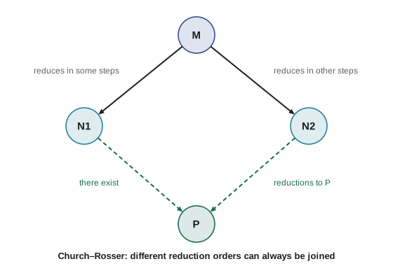
Two theorems govern the choices. The Church–Rosser theorem, also called confluence, says that if a term reduces to two different terms, both can be reduced further to a common term. A consequence is that a term has at most one normal form, whatever order we use to find it. The standardization theorem says that if a term has a normal form, normal-order reduction will find it. Applicative order can loop where normal order succeeds, as the next example shows: (λx.y) Ω has normal form y, but applicative order evaluates Ω first and never stops.

# Normal order versus applicative order on (\x.y) Omega, where Omega = (\x.x x)(\x.x x).
# Applicative order evaluates the argument first and loops; normal order discards it.
omega = "(\u03bbx.x x)(\u03bbx.x x)"
# one beta step substitutes (\u03bbx.x x) for x in "x x", which rebuilds the same term
print("Omega steps to:", omega, "(itself, so reduction never ends)")
print("normal order on (\u03bbx.y) \u03a9: one step -> y        (argument never evaluated)")
print("applicative order on (\u03bbx.y) \u03a9: evaluate \u03a9 first -> \u03a9 -> \u03a9 -> ... (no end)")

# Python is applicative: arguments are evaluated before the call.
import sys
sys.setrecursionlimit(200)
def omega(): return omega()
def const_y(x): return "y"
try:
    const_y(omega())
except RecursionError:
    print("Python const_y(omega()): RecursionError, because Python evaluates the argument first")
print("Delaying the argument with a thunk works:", (lambda thunk: "y")(lambda: omega()))

Omega steps to: (λx.x x)(λx.x x) (itself, so reduction never ends)
normal order on (λx.y) Ω: one step -> y        (argument never evaluated)
applicative order on (λx.y) Ω: evaluate Ω first -> Ω -> Ω -> ... (no end)
Python const_y(omega()): RecursionError, because Python evaluates the argument first
Delaying the argument with a thunk works: y

Programming with only functions

With nothing but functions we can encode data. Church numerals represent the number n as the function that applies f to x n times: 0 is λf x.x, 1 is λf x.f x, 2 is λf x.f (f x). The successor function adds one more application: succ = λn f x.f (n f x). Addition applies f m times on top of n applications, and multiplication composes. Booleans are functions that choose: true = λa b.a and false = λa b.b, so 'if c then t else e' is simply c t e. Pairs store two values and hand them to a selector function. The predecessor function is famously awkward; Stephen Kleene is said to have found the trick while at the dentist, by sliding a pair (n − 1, n) along.

# Church encodings: numbers, booleans and pairs built from functions alone.
zero  = lambda f: lambda x: x
succ  = lambda n: lambda f: lambda x: f(n(f)(x))
plus  = lambda m: lambda n: lambda f: lambda x: m(f)(n(f)(x))
times = lambda m: lambda n: lambda f: m(n(f))
power = lambda m: lambda n: n(m)
to_int = lambda n: n(lambda k: k + 1)(0)          # decode by counting applications

one, two = succ(zero), succ(succ(zero))
three = plus(one)(two)
print("3       =", to_int(three))
print("2 * 3   =", to_int(times(two)(three)))
print("2 ^ 3   =", to_int(power(two)(three)))

true  = lambda a: lambda b: a
false = lambda a: lambda b: b
if_   = lambda c: lambda t: lambda e: c(t)(e)
is_zero = lambda n: n(lambda _: false)(true)
print("is_zero(0), is_zero(2):", if_(is_zero(zero))("yes")("no"), if_(is_zero(two))("yes")("no"))

pair = lambda a: lambda b: lambda sel: sel(a)(b)
fst, snd = lambda p: p(true), lambda p: p(false)
# predecessor by sliding a pair (n-1, n) along: Kleene's trick
pred = lambda n: fst(n(lambda p: pair(snd(p))(succ(snd(p))))(pair(zero)(zero)))
print("pred(3) =", to_int(pred(three)))

3       = 3
2 * 3   = 6
2 ^ 3   = 8
is_zero(0), is_zero(2): yes no
pred(3) = 2

These encodings are not how real languages represent numbers, but they prove a point: functions alone are enough to express any computation. They also reappear in practice. The visitor pattern in object-oriented languages and the fold functions in functional languages are Church encodings of data structures under different names.

Recursion without names

The lambda calculus has no way for a function to refer to itself by name, yet it can express recursion. A fixed-point combinator Y satisfies Y F = F (Y F) for every F. To define factorial, write a non-recursive function F that takes the recursive call as an extra parameter, F = λself n.if n = 0 then 1 else n × self (n − 1), and let fact = Y F. Unfolding Y F gives F (Y F), so self is bound to fact itself. Haskell Curry's Y combinator is Y = λf.(λx.f (x x))(λx.f (x x)). Under applicative order, Y loops before ever calling F, so strict languages use the Z combinator, which wraps the self-application in an extra lambda to delay it.

# Recursion without names: fixed-point combinators.
# Y = \f.(\x.f (x x))(\x.f (x x)) loops under applicative order, so strict languages
# use the Z combinator, which delays the self-application with an extra lambda.
Z = lambda f: (lambda x: f(lambda v: x(x)(v)))(lambda x: f(lambda v: x(x)(v)))

fact_step = lambda self: lambda n: 1 if n == 0 else n * self(n - 1)
fib_step  = lambda self: lambda n: n if n < 2 else self(n - 1) + self(n - 2)

fact, fib = Z(fact_step), Z(fib_step)
print("fact 10 =", fact(10))
print("fib 0..10 =", [fib(i) for i in range(11)])
# A fixed point: fact_step(fact) behaves exactly like fact.
print("fact_step(fact)(6) == fact(6):", fact_step(fact)(6) == fact(6))

fact 10 = 3628800
fib 0..10 = [0, 1, 1, 2, 3, 5, 8, 13, 21, 34, 55]
fact_step(fact)(6) == fact(6): True

Fixed points also connect back to lesson 3: the meaning of a while loop was defined as the least fixed point of a functional, and Y builds exactly such fixed points at the level of terms. In practice, languages provide recursion directly with letrec, def or let rec, and compilers implement it with the environment cycle from lesson 4, but the combinator shows that recursion is not an extra primitive.

Implementing substitution efficiently

Renaming variables to avoid capture is error-prone and slow. Nicolaas de Bruijn proposed replacing each bound variable by a number: how many binders lie between the variable and the binder that introduces it. λx.λy.x becomes λ λ 1 and λx.x becomes λ 0. Alpha-equivalent terms then have identical representations, so equality is a simple structural comparison and capture cannot happen. De Bruijn indices are used inside proof assistants such as Coq and Lean, and in many compilers' intermediate representations.

# de Bruijn indices: replace each bound variable by the number of binders between it
# and the binder that introduces it.  Alpha-equivalent terms get identical representations.
def to_db(t, ctx=()):
    if t[0] == "var":
        return ctx.index(t[1]) if t[1] in ctx else t[1]     # free variables keep their names
    if t[0] == "lam":
        return ("\u03bb", to_db(t[2], (t[1],) + ctx))
    return ("@", to_db(t[1], ctx), to_db(t[2], ctx))

K1 = ("lam", "x", ("lam", "y", ("var", "x")))              # \x.\y.x
K2 = ("lam", "a", ("lam", "b", ("var", "a")))              # \a.\b.a
S  = ("lam", "f", ("lam", "g", ("lam", "x",
      ("app", ("app", ("var", "f"), ("var", "x")), ("app", ("var", "g"), ("var", "x"))))))
print("\u03bbx.\u03bby.x  ->", to_db(K1))
print("\u03bba.\u03bbb.a  ->", to_db(K2))
print("alpha-equivalent:", to_db(K1) == to_db(K2))
print("S combinator ->", to_db(S))

λx.λy.x  -> ('λ', ('λ', 1))
λa.λb.a  -> ('λ', ('λ', 1))
alpha-equivalent: True
S combinator -> ('λ', ('λ', ('λ', ('@', ('@', 2, 0), ('@', 1, 0)))))

Why the lambda calculus matters

The Church–Turing thesis states that every effectively computable function can be computed by a Turing machine, or equivalently by a lambda term; the two models were shown equivalent in 1937. For language designers, the lambda calculus is a laboratory. Add types and you get the simply typed lambda calculus of lesson 7, in which every program terminates. Add polymorphism and inference and you get the core of ML and Haskell (lesson 8). Add references and you get a model of imperative languages. Peter Landin argued in 1966 that every programming language could be understood as lambda calculus plus some extras, and modern compilers for functional languages still translate source programs into a lambda-calculus-like core before optimizing them.

Worked examples