
CMPUT-204 · Lesson 12 of 12 · 25 min
Capstone: designing and analysing algorithms for a real problem
This final lesson puts the course to work. Real problems do not arrive labelled as sorting or shortest paths; they arrive as messy requirements from people who need software. The skill that matters most is recognizing the classic problems hidden inside, choosing algorithms with the right guarantees, and estimating costs before writing code. The lesson first adds one more analytical tool, amortized analysis, then works through an invented case study, a courier company, from requirements to analysed design, and closes with the gap between asymptotic analysis and real performance, and with what comes next in CMPUT-304.
Amortized analysis
Some operations are usually cheap but occasionally expensive. A growable array, such as a Python list or the dynamic array from CMPUT-201 lesson 9, stores items in a fixed-size block; when the block is full, it allocates a block twice as large and copies everything over. A single append can therefore cost \(\Theta(n)\). But expensive appends are rare, and amortized analysis bounds the total cost of a whole sequence of operations, then divides by the number of operations. It is a worst-case guarantee about sequences, not an average over random inputs.
The aggregate method adds up the total cost directly. Starting from capacity 1 and doubling, \(n\) appends trigger copies of \(1, 2, 4, \ldots\) items, up to the largest power of two below \(n\). That geometric series, lesson 3's favourite pattern, sums to less than \(2n\). Adding the \(n\) writes of the new items, the total is less than \(3n\), so each append costs \(O(1)\) amortized. The accounting method gives the same answer with a story: charge each append 3 units, spend 1 on writing the item, and save 2 as credit. When the array of capacity \(k\) fills and must be copied, the \(k/2\) items added since the last doubling have saved \(k\) units, exactly enough to pay for copying all \(k\) items.
def copies(n, grow):
    cap, size, copied = 1, 0, 0
    for _ in range(n):
        if size == cap:
            copied += size                  # move every item to the new block
            cap = grow(cap)
        size += 1
    return copied

for n in (1000, 100000, 1000000):
    d = copies(n, lambda c: 2 * c)
    a = copies(n, lambda c: c + 100) if n <= 100000 else None
    line = f'n={n:>8}: doubling copies {d:>8} ({d / n:.2f} per append)'
    if a is not None:
        line += f', grow by 100 copies {a:>10} ({a / n:.1f} per append)'
print(line)n= 1000: doubling copies 1023 (1.02 per append), grow by 100 copies 4510 (4.5 per append) n= 100000: doubling copies 131071 (1.31 per append), grow by 100 copies 49951000 (499.5 per append) n= 1000000: doubling copies 1048575 (1.05 per append)
Doubling copies between about 1.0 and 1.3 items per append at every size, always under the bound of 2, while growing by a fixed 100 slots copies about 500 items per append at \(n = 100{,}000\), because that is an arithmetic series with \(\Theta(n^2)\) total cost. The lesson for designers is that geometric growth, by any constant factor greater than 1, gives constant amortized time; CPython actually grows lists by about 12.5 per cent plus a small constant to save memory. Amortized analysis also explains the near-constant cost of union–find operations in lesson 10.
The case study: Aspen Valley Couriers
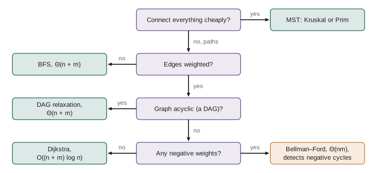
Aspen Valley Couriers is an invented same-day delivery company in a mid-sized city. Each morning it receives a list of parcels, each with a destination and a delivery time window, and it must plan the day. The operations manager describes five needs. First, the travel time from the depot to every delivery address, over a road network with about 40,000 intersections and 100,000 road segments, each with a travel time in minutes. Second, how many vans are needed so that every delivery window is covered without one van being in two places at once. Third, an order for the morning loading tasks, some of which depend on others. Fourth, a list of the 50 most urgent parcels each hour, from a few thousand. Fifth, a plan for laying a private radio-relay network between the company's 30 pickup lockers at minimum cost.
| Need | Classic problem hidden inside | Algorithm | Lesson |
|---|---|---|---|
| Travel times from the depot | Single-source shortest paths, non-negative weights | Dijkstra with a binary heap | 9 |
| Number of vans for time windows | Interval partitioning | Greedy by start time with a heap | 11 |
| Order of loading tasks | Topological sort of a DAG | Kahn's algorithm, reporting cycles | 8 |
| 50 most urgent parcels | Selection or partial sorting | Heap of size 50, or quickselect then sort 50 | 5, 6 |
| Radio-relay network between lockers | Minimum spanning tree | Kruskal with union–find | 10 |
Analysing the design before coding
With \(n = 40{,}000\) intersections and \(m = 100{,}000\) road segments, Dijkstra with a binary heap performs on the order of \((n + m)\log_2 n \approx 140{,}000 \times 15.3 \approx 2.1\) million basic heap steps, well under a second even in Python. A Bellman–Ford run would be about \(n \times m = 4 \times 10^9\) relaxations, which in Python could take over an hour; since travel times are never negative, Dijkstra is both correct and far faster. Storing the network as an adjacency matrix would need \(1.6 \times 10^9\) cells, so adjacency lists are essential.
For the vans, \(k\) parcels with windows sort in \(O(k \log k)\), and the greedy assignment uses exactly as many vans as the maximum number of overlapping windows, which the depth computation from lesson 11 confirms. The urgent-parcel report keeps a min-heap of the 50 most urgent seen so far while scanning \(k\) parcels, costing \(O(k \log 50)\), essentially linear, instead of sorting all \(k\). The relay network has only 30 lockers, so \(30 \times 29 / 2 = 435\) candidate links; Kruskal handles that instantly. Each design choice comes with a guarantee: correctness from the lesson's proof and a running time from its analysis.
import heapq, random
from collections import deque

random.seed(204)
# --- a small synthetic road grid: 30 x 30 intersections, travel times 1-5 minutes ---
W = H = 30
adj = {(x, y): [] for x in range(W) for y in range(H)}
for x in range(W):
    for y in range(H):
        for dx, dy in ((1, 0), (0, 1)):
            nx, ny = x + dx, y + dy
            if nx < W and ny < H:
                t = random.randint(1, 5)
                adj[(x, y)].append(((nx, ny), t)); adj[(nx, ny)].append(((x, y), t))

def dijkstra(src):
    dist, pq, done = {src: 0}, [(0, src)], set()
    while pq:
        d, u = heapq.heappop(pq)
        if u in done: continue
        done.add(u)
        for v, w in adj[u]:
            if d + w < dist.get(v, 10**9):
                dist[v] = d + w; heapq.heappush(pq, (dist[v], v))
    return dist

depot = (15, 15)
dist = dijkstra(depot)
stops = random.sample(sorted(adj), 8)
print('travel minutes from depot:', [dist[s] for s in stops])

# --- vans needed for delivery windows (start, end) in minutes after 8:00 ---
windows = []
for _ in range(60):
    s = random.randint(0, 480); windows.append((s, s + random.randint(30, 120)))
vans = []
for s, e in sorted(windows):
    if vans and vans[0] <= s: heapq.heapreplace(vans, e)
    else: heapq.heappush(vans, e)
print('vans needed:', len(vans))

# --- loading tasks with dependencies (Kahn) ---
deps = {'unlock bay': ['scan parcels'], 'scan parcels': ['sort by route'], 'charge vans': ['load vans'],
        'sort by route': ['load vans'], 'load vans': ['print manifests'], 'print manifests': []}
indeg = {t: 0 for t in deps}
for t in deps:
    for u in deps[t]: indeg[u] += 1
q, order = deque(t for t in deps if indeg[t] == 0), []
while q:
    t = q.popleft(); order.append(t)
    for u in deps[t]:
        indeg[u] -= 1
        if indeg[u] == 0: q.append(u)
print('loading order:', ' > '.join(order))

# --- the 5 most urgent of 3,000 parcels (minutes until deadline) ---
urgency = [random.randint(10, 600) for _ in range(3000)]
print('most urgent:', heapq.nsmallest(5, urgency))travel minutes from depot: [42, 15, 11, 42, 42, 34, 30, 34] vans needed: 15 loading order: unlock bay > charge vans > scan parcels > sort by route > load vans > print manifests most urgent: [10, 10, 11, 11, 11]
The miniature system runs each component on synthetic data in a fraction of a second. In production, the components would read real map data and parcel records, but the algorithms, and their guarantees, would be the same. heapq.nsmallest uses the bounded-heap method described above.
A problem the course cannot solve efficiently
The manager's sixth request is the hardest: plan the order in which each van visits its stops to minimize total driving time. That is the travelling salesperson problem, and no efficient algorithm for it is known. Trying every order of 20 stops means \(20!/2 \approx 1.2 \times 10^{18}\) routes. The problem is NP-hard, a notion made precise in CMPUT-304, which means a polynomial-time exact algorithm would also solve thousands of other problems believed to be hard. Recognizing such problems is as important as solving easy ones, because it redirects effort to the right kind of solution: exact methods for small instances, approximation algorithms with proven guarantees, such as the MST-based tour within twice the optimum mentioned in lesson 10, or heuristics that work well in practice.
Worked problem
Estimating before building
A developer proposes computing travel times between every pair of the 40,000 intersections each morning by running Dijkstra from each one. Is that feasible?
Show solution
- One Dijkstra run costs about 2.1 million heap steps, as estimated above.
- 40,000 runs cost about 40,000 × 2.1 × 10⁶ ≈ 8.4 × 10¹⁰ steps.
- At roughly 10⁷ simple Python steps per second, that is around 8,400 seconds, more than two hours, and the result has 1.6 × 10⁹ entries.
- Only distances among the depot and that day's few hundred stops are needed: a few hundred Dijkstra runs take minutes and produce a table of about 10⁵ entries.
Answer: All-pairs is wasteful; compute distances only from the depot and the day's stops. A two-minute estimate saved a two-hour job.
When constants and hardware matter
Asymptotic analysis is the first word on performance, not the last. Constant factors decide between algorithms with the same growth rate: quicksort usually beats heapsort because its inner loop is tighter and it scans memory sequentially, and modern processors reward sequential access through caches that can make it ten or more times faster than random access. Thresholds matter too: library sorts switch to insertion sort for subarrays of about 16 to 64 items, because below that size its low overhead beats any \(n \log n\) method. Measure with doubling experiments, as in lesson 1, and profile real workloads before optimizing.
| Situation | Practical consideration | Typical response |
|---|---|---|
| Small n | Constant factors dominate | Use simple algorithms, or hybrid algorithms with a cut-off |
| Huge data on disk | Disk and network access dominate | External merge sort, sequential access, batching |
| Adversarial inputs | Worst cases are deliberately triggered | Randomized pivots, worst-case guarantees, hashing with random seeds |
| Many repeated queries | Precomputation can pay off | Sort once, build indexes, cache results |
| NP-hard problem | No known efficient exact algorithm | Approximation algorithms and heuristics (CMPUT-304) |
Where to go next
This course covered the core of algorithm design: analysis, sorting, divide and conquer, graph search, shortest paths, spanning trees and greedy methods. CMPUT-304 continues with dynamic programming, which handles the overlapping subproblems that defeat divide and conquer and solves 0/1 knapsack and all-pairs shortest paths; network flow and matching; NP-completeness; and approximation and randomized algorithms. CMPUT-474 studies what can be computed at all. Algorithms also run through the rest of the program: query processing in CMPUT-291, routing in CMPUT-313, search in CMPUT-366 and path planning in the robotics courses. Wherever they appear, the habits from this course apply: state the problem precisely, prove the algorithm correct, analyse its cost, and measure.
Common mistakes
MistakeCalling an operation O(1) amortized because it is usually fast.
InsteadAmortized bounds are proved for every sequence of operations, by the aggregate or accounting method, not from typical behaviour.
MistakeGrowing an array by a constant number of slots.
InsteadConstant growth gives Θ(n²) total copying; grow by a constant factor for O(1) amortized appends.
MistakeStarting to code before identifying the classic problem inside a requirement.
InsteadMap each requirement to a known problem first; the right algorithm and its guarantees follow.
MistakeComputing far more than the task needs, such as all-pairs distances.
InsteadEstimate costs first and compute only what is required.
MistakeTreating an NP-hard problem as if a clever exact algorithm must exist.
InsteadRecognize hardness early and choose approximations or heuristics with known behaviour.
Summary and key terms
- Amortized analysis bounds the total cost of any sequence of operations; doubling a dynamic array makes appends O(1) amortized.
- The aggregate method sums costs directly; the accounting method prepays expensive operations with saved credit.
- Real requirements hide classic problems: shortest paths, interval partitioning, topological sort, selection and spanning trees.
- Back-of-the-envelope estimates using asymptotic bounds and real sizes reveal infeasible designs before any code is written.
- Some problems, such as the travelling salesperson problem, are NP-hard and call for approximation or heuristics.
- Constant factors, caches and thresholds decide between algorithms with the same growth rate; measure to confirm.
- CMPUT-304 continues with dynamic programming, network flow, NP-completeness and randomized algorithms.
- Amortized cost
- The total cost of a sequence of operations divided by the number of operations, bounded in the worst case.
- Aggregate method
- Amortized analysis by bounding the total cost of n operations directly.
- Accounting method
- Amortized analysis that charges extra on cheap operations to pay for expensive ones.
- Dynamic array
- An array that grows by allocating a larger block and copying when it fills.
- Geometric growth
- Increasing capacity by a constant factor greater than 1.
- Problem reduction
- Recognizing that a new problem is an instance of a known one.
- Back-of-the-envelope estimate
- A quick calculation of resource needs from asymptotic bounds and real sizes.
- NP-hard
- At least as hard as every problem in NP; no polynomial-time algorithm is known.
- Approximation algorithm
- An efficient algorithm whose solution is guaranteed to be within a factor of optimal.
- Hybrid algorithm
- An algorithm that switches methods by input size, such as quicksort with an insertion-sort cut-off.
Practice problems
Work each problem on paper first, then reveal the answer to check.
With doubling from capacity 1, how many items are copied in total over 16 appends?
Show answer
1 + 2 + 4 + 8 = 15 copies.
Under the accounting method, why is a charge of 3 per append enough?
Show answer
One unit writes the item; two units saved per item since the last doubling pay to copy the whole array at the next doubling.
Why does growing by 100 slots give quadratic total cost?
Show answer
Copies of 100, 200, 300, ... items form an arithmetic series of about n²/200 total.
A city has 10⁶ intersections and 2.5 × 10⁶ road segments. Estimate one Dijkstra run.
Show answer
About 3.5 × 10⁶ × 20 ≈ 7 × 10⁷ heap steps.
Which algorithm assigns delivery windows to the fewest vans?
Show answer
Greedy interval partitioning by start time with a heap of finish times.
Why is Bellman–Ford the wrong choice for travel times?
Show answer
Travel times are non-negative, so Dijkstra is correct and much faster than Θ(nm).
How would you report the 50 most urgent of k parcels efficiently?
Show answer
Scan once keeping a heap of the 50 best, O(k log 50); or quickselect then sort 50.
What kind of problem is ordering a van's stops to minimize driving?
Show answer
The travelling salesperson problem, which is NP-hard.
Name two reasons quicksort often beats heapsort despite equal asymptotic bounds.
Show answer
A tighter inner loop with fewer comparisons, and sequential memory access that suits caches.
List the four habits this course recommends for any algorithmic task.
Show answer
State the problem precisely, prove the algorithm correct, analyse its cost, and measure.
Lesson quiz · 5 questions
Score 60% or more to complete this lesson.
Create a free account to save your progress, take quizzes and earn a certificate.