
CMPUT-204 · Lesson 10 of 12 · 30 min
Minimum spanning trees and union–find
Suppose a town wants to connect several buildings with fibre-optic cable, and each possible link has a cost. The cheapest network that connects everything is a minimum spanning tree. This lesson proves the two properties that make minimum spanning trees easy to find, then develops the two classic algorithms: Kruskal's, which adds the cheapest safe edges in sorted order using a union–find data structure, and Prim's, which grows a single tree with a priority queue. Both run in \(O(m \log n)\) time, and both are greedy algorithms whose correctness rests on a precise argument rather than luck.
Spanning trees and the problem
Let \(G = (V, E)\) be a connected, undirected graph with a weight \(w(e)\) on each edge. A spanning tree is a subset of edges that connects all \(n\) vertices and contains no cycle; by the tree facts from CMPUT-272 lesson 12, it has exactly \(n - 1\) edges. A minimum spanning tree, or MST, is a spanning tree with the smallest total weight. A graph can have exponentially many spanning trees, \(n^{n-2}\) of them for a complete graph on \(n\) vertices by Cayley's formula, so trying them all is hopeless. Fortunately, a simple greedy strategy is guaranteed to work.
The cut property and the cycle property
A cut of the graph is a partition of the vertices into two non-empty sets \(S\) and \(V \setminus S\). An edge crosses the cut if it has one endpoint on each side. The cut property says: for any cut, a lightest edge crossing it belongs to some minimum spanning tree, and if it is the unique lightest crossing edge, it belongs to every MST. The proof is an exchange argument. Take any MST \(T\) that does not contain the lightest crossing edge \(e = \{u, v\}\). Adding \(e\) to \(T\) creates a cycle, and that cycle must cross the cut a second time at some other edge \(f\). Removing \(f\) gives another spanning tree whose weight is \(w(T) + w(e) - w(f) \le w(T)\), because \(w(e) \le w(f)\). So there is an MST containing \(e\).
The cycle property is the mirror image: the heaviest edge on any cycle, if it is unique, belongs to no MST, because removing it from a tree that contains it and reconnecting with a lighter edge of the cycle would reduce the weight. Together these properties say that both adding the cheapest safe edge and discarding the most expensive redundant edge are always safe moves. When all edge weights are distinct, the MST is unique.
Worked problem
Applying the cut property
In a graph, the cut separating {A, B} from the other vertices is crossed by edges A–C (4), B–C (2) and B–D (7). Which edge must be in every MST, assuming distinct weights?
Show solution
- List the crossing edges and their weights: 4, 2 and 7.
- The unique lightest crossing edge is B–C with weight 2.
- By the cut property, B–C belongs to every minimum spanning tree.
- Nothing yet can be said about A–C or B–D from this cut alone.
Answer: B–C. Each greedy step in Kruskal and Prim is justified by finding a cut for which the chosen edge is the lightest crossing edge.
Kruskal's algorithm
Kruskal's algorithm sorts the edges by weight and examines them from lightest to heaviest. It adds an edge to the forest it is building if the edge joins two different trees, and skips it if both endpoints are already in the same tree, because adding it would create a cycle. When \(n - 1\) edges have been added, the forest is a spanning tree. Each added edge is the lightest edge crossing the cut between the tree containing one endpoint and the rest of the graph, so the cut property shows the result is an MST.
The only difficult step is deciding quickly whether two vertices are already in the same tree. Searching the forest with BFS for every edge would cost \(O(n)\) per edge and \(O(nm)\) in total. A specialized data structure answers the question in nearly constant time.
The union–find data structure
Union–find, also called a disjoint-set structure, maintains a collection of disjoint sets with two operations: find\((x)\) returns a representative of the set containing \(x\), so two items are in the same set exactly when their finds are equal; and union\((x, y)\) merges their two sets. It stores each set as a rooted tree using a parent array, with each root as its set's representative. Find follows parent pointers to the root; union makes one root the parent of the other.
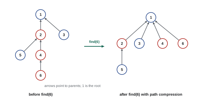
Without care the trees can become long chains, making find take \(\Theta(n)\). Two simple heuristics fix this. Union by rank attaches the shorter tree under the taller one, which alone keeps every tree's height at most \(\log_2 n\), because a tree's height grows only when two trees of equal height merge, and that doubles the minimum size. Path compression makes every node visited during a find point directly to the root, flattening the tree for future finds. With both heuristics, a sequence of \(m\) operations on \(n\) items takes \(O(m\, \alpha(n))\) time, where \(\alpha\) is the inverse Ackermann function, which is at most 4 for any input that could fit in the universe. For practical purposes each operation costs constant amortized time.
class UnionFind:
    def __init__(self, items):
        self.parent = {x: x for x in items}
        self.rank = {x: 0 for x in items}
        self.steps = 0                         # parent pointers followed, for analysis
    def find(self, x):
        root = x
        while self.parent[root] != root:
            root = self.parent[root]; self.steps += 1
        while self.parent[x] != root:          # path compression
            self.parent[x], x = root, self.parent[x]
        return root
    def union(self, x, y):
        rx, ry = self.find(x), self.find(y)
        if rx == ry:
            return False
        if self.rank[rx] < self.rank[ry]:      # union by rank
            rx, ry = ry, rx
        self.parent[ry] = rx
        if self.rank[rx] == self.rank[ry]:
            self.rank[rx] += 1
        return True

import random
random.seed(10)
n = 100000
uf = UnionFind(range(n))
ops = 0
for _ in range(3 * n):
    a, b = random.randrange(n), random.randrange(n)
    uf.union(a, b); ops += 1
sets = len({uf.find(x) for x in range(n)})
print('sets remaining:', sets)
print('average pointer steps per find:', round(uf.steps / (2 * ops + n), 3))
print('maximum rank:', max(uf.rank.values()), ' log2 n =', round(n.bit_length() - 1))sets remaining: 244 average pointer steps per find: 0.932 maximum rank: 7 log2 n = 16
After 300,000 random unions on 100,000 items, the average find follows fewer than one parent pointer, and the largest rank is only 7, far below the guaranteed bound of \(\log_2 n \approx 16\). Union–find appears far beyond MSTs: in image segmentation, in compilers that unify types, in detecting connected components of a graph that grows over time, and in percolation simulations.
import heapq

class UnionFind:                               # compact version of the class above
    def __init__(self, items):
        self.parent = {x: x for x in items}; self.rank = {x: 0 for x in items}
    def find(self, x):
        while self.parent[x] != x:
            self.parent[x] = self.parent[self.parent[x]]   # path halving
            x = self.parent[x]
        return x
    def union(self, x, y):
        rx, ry = self.find(x), self.find(y)
        if rx == ry: return False
        if self.rank[rx] < self.rank[ry]: rx, ry = ry, rx
        self.parent[ry] = rx
        self.rank[rx] += self.rank[rx] == self.rank[ry]
        return True

def kruskal(vertices, edges):
    uf = UnionFind(vertices)
    tree, total = [], 0
    for w, u, v in sorted(edges):              # Theta(m log m) sort dominates
        if uf.union(u, v):
            tree.append((u, v, w)); total += w
            if len(tree) == len(vertices) - 1:
                break
    return total, tree

def prim(vertices, edges, start):
    adj = {v: [] for v in vertices}
    for w, u, v in edges:
        adj[u].append((w, v)); adj[v].append((w, u))
    in_tree, total, tree = {start}, 0, []
    pq = [(w, start, v) for w, v in adj[start]]
    heapq.heapify(pq)
    while pq and len(in_tree) < len(vertices):
        w, u, v = heapq.heappop(pq)
        if v in in_tree:
            continue                           # stale: both ends already in the tree
        in_tree.add(v); total += w; tree.append((u, v, w))
        for w2, x in adj[v]:
            if x not in in_tree:
                heapq.heappush(pq, (w2, v, x))
    return total, tree

V = list('ABCDEFG')
E = [(7, 'A', 'B'), (5, 'A', 'D'), (8, 'B', 'C'), (9, 'B', 'D'), (7, 'B', 'E'), (5, 'C', 'E'),
     (15, 'D', 'E'), (6, 'D', 'F'), (8, 'E', 'F'), (9, 'E', 'G'), (11, 'F', 'G')]
tk, treek = kruskal(V, E)
tp, treep = prim(V, E, 'A')
print('Kruskal:', tk, sorted((min(u, v) + max(u, v), w) for u, v, w in treek))
print('Prim :', tp, sorted((min(u, v) + max(u, v), w) for u, v, w in treep))Kruskal: 39 [('AB', 7), ('AD', 5), ('BE', 7), ('CE', 5), ('DF', 6), ('EG', 9)]
Prim : 39 [('AB', 7), ('AD', 5), ('BE', 7), ('CE', 5), ('DF', 6), ('EG', 9)]Prim's algorithm
Prim's algorithm grows one tree from a starting vertex. At each step it adds the lightest edge that connects a vertex in the tree to a vertex outside it. That edge is the lightest crossing the cut between the tree and everything else, so the cut property makes every step safe. A priority queue holds candidate edges, or equivalently, for each outside vertex, the cheapest known edge into the tree. With a binary heap the algorithm runs in \(O(m \log n)\), like Dijkstra's algorithm, which it closely resembles: Dijkstra keys a vertex by its distance from the source, while Prim keys it by the weight of a single connecting edge.
| Property | Kruskal | Prim |
|---|---|---|
| Grows | A forest that merges into one tree | A single tree from a start vertex |
| Chooses | Lightest edge that joins two trees | Lightest edge leaving the tree |
| Key data structure | Union–find | Priority queue (binary heap) |
| Running time | O(m log m) = O(m log n), dominated by sorting | O(m log n) with a binary heap; O(n²) with an array |
| Works well for | Sparse graphs, edges already sorted, clustering | Dense graphs (array version), graphs given by adjacency |
| Correctness argument | Cut property on the two merged trees | Cut property on the current tree |
Worked problem
The first steps of Kruskal
Using the edge list in the code above, which edges does Kruskal add first, and which does it skip?
Show solution
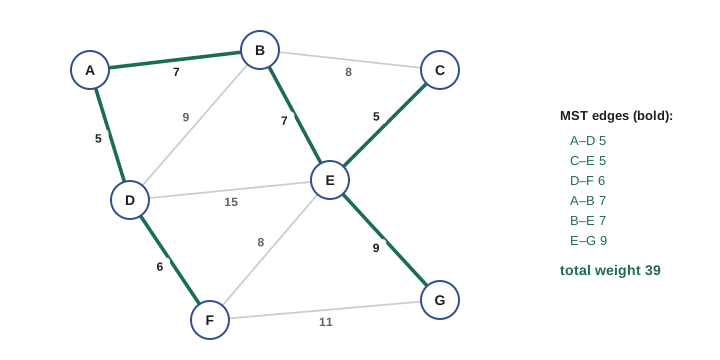
- Sorted, the lightest edges are A–D (5), C–E (5), D–F (6), A–B (7), B–E (7), B–C (8), E–F (8), ...
- Add A–D, C–E and D–F: each joins two different trees.
- Add A–B (7), joining B to the tree {A, D, F}; add B–E (7), joining that tree to {C, E}.
- Skip B–C (8) and E–F (8): their endpoints are already connected. Add E–G (9) to reach all 7 vertices.
Answer: The tree is A–D, C–E, D–F, A–B, B–E, E–G with total weight 39, the value both algorithms print.
Applications of minimum spanning trees
MSTs solve network design directly: cable, pipeline and road networks where the goal is the cheapest way to connect everything. They also appear inside other algorithms. Stopping Kruskal's algorithm when \(k\) trees remain divides the vertices into \(k\) clusters with the largest possible minimum distance between clusters, a method called single-linkage clustering used in data analysis and biology. For the travelling salesperson problem with distances that obey the triangle inequality, walking around an MST gives a tour at most twice the optimal length, an approximation algorithm discussed in CMPUT-304. Image segmentation, handwriting recognition and the design of electrical grids all use MSTs as building blocks.
import random, math

class UnionFind:                               # compact version of the class above
    def __init__(self, items):
        self.parent = {x: x for x in items}; self.rank = {x: 0 for x in items}
    def find(self, x):
        while self.parent[x] != x:
            self.parent[x] = self.parent[self.parent[x]]   # path halving
            x = self.parent[x]
        return x
    def union(self, x, y):
        rx, ry = self.find(x), self.find(y)
        if rx == ry: return False
        if self.rank[rx] < self.rank[ry]: rx, ry = ry, rx
        self.parent[ry] = rx
        self.rank[rx] += self.rank[rx] == self.rank[ry]
        return True

random.seed(11)
pts = [(random.gauss(cx, 0.6), random.gauss(cy, 0.6))
       for cx, cy in ((0, 0), (6, 1), (3, 6)) for _ in range(15)]
idx = list(range(len(pts)))
edges = sorted((math.dist(pts[i], pts[j]), i, j) for i in idx for j in idx if i < j)
uf = UnionFind(idx)
groups = len(idx)
for w, i, j in edges:
    if groups == 3:
        break                                  # stop Kruskal with k = 3 trees left
    if uf.union(i, j):
        groups -= 1
labels = {}
for i in idx:
    labels.setdefault(uf.find(i), []).append(i)
sizes = sorted(len(v) for v in labels.values())
print('cluster sizes:', sizes)
print('each true group recovered:', sorted(sorted(v)[0] // 15 for v in labels.values()) == [0, 1, 2]
and all(len({i // 15 for i in v}) == 1 for v in labels.values()))cluster sizes: [15, 15, 15] each true group recovered: True
Common mistakes
MistakeThinking the MST gives shortest paths between vertices.
InsteadAn MST minimizes total edge weight; the path between two vertices in the MST can be much longer than their shortest path.
MistakeChecking for cycles in Kruskal by searching the forest each time.
InsteadUse union–find: two vertices are in the same tree exactly when their finds agree.
MistakeImplementing union–find without union by rank or path compression.
InsteadTrees can become chains with Θ(n) finds; the two heuristics give near-constant amortized time.
MistakeApplying MST algorithms to directed graphs.
InsteadMSTs are defined for undirected graphs; the directed analogue, minimum arborescence, needs a different algorithm.
MistakeAssuming the MST is unique when weights repeat.
InsteadWith equal weights there may be several MSTs, all with the same total weight.
Summary and key terms
- A spanning tree connects all n vertices with n − 1 edges and no cycle; an MST has minimum total weight.
- Cut property: a lightest edge crossing any cut belongs to some MST.
- Cycle property: a unique heaviest edge on a cycle belongs to no MST.
- Kruskal's algorithm adds edges in increasing weight order when they join two different trees, in O(m log n).
- Union–find with union by rank and path compression supports find and union in O(α(n)) amortized time.
- Prim's algorithm grows one tree, always adding the lightest edge leaving it, in O(m log n) with a binary heap.
- MSTs solve network design and underlie single-linkage clustering and approximation algorithms.
- Spanning tree
- A tree containing every vertex of a connected graph.
- Minimum spanning tree
- A spanning tree of minimum total edge weight.
- Cut
- A partition of the vertices into two non-empty sets.
- Crossing edge
- An edge with one endpoint on each side of a cut.
- Cut property
- A lightest crossing edge of any cut is in some MST.
- Union–find
- A data structure for disjoint sets supporting find and union.
- Union by rank
- Attaching the root of the shorter tree under the root of the taller one.
- Path compression
- Making nodes visited by find point directly to the root.
- Inverse Ackermann function
- α(n), a function that grows so slowly it is at most 4 for all practical n.
- Single-linkage clustering
- Grouping points by stopping Kruskal's algorithm when k trees remain.
Practice problems
Work each problem on paper first, then reveal the answer to check.
How many edges does a spanning tree of a 50-vertex graph have?
Show answer
49.
How many spanning trees does the complete graph on 4 vertices have?
Show answer
4⁴⁻² = 16, by Cayley's formula.
In Kruskal, edge (u, v) is next and find(u) = find(v). What happens?
Show answer
The edge is skipped because it would create a cycle.
What is the maximum height of a union–find tree with union by rank on 1,024 items?
Show answer
log₂ 1024 = 10.
Why does Kruskal's running time come out to O(m log n)?
Show answer
Sorting m edges costs O(m log m), and log m ≤ 2 log n; union–find operations add only O(m α(n)).
Which algorithm would you choose for a dense graph given as an adjacency matrix?
Show answer
Prim with an array-based priority queue, which runs in Θ(n²).
A cycle has edge weights 3, 8, 5, 11. Which edge can never be in an MST?
Show answer
The edge of weight 11, the unique heaviest edge on the cycle.
Add 10 to every edge weight. Does the MST change?
Show answer
No: every spanning tree gains 10(n − 1), so the order of trees by weight is unchanged.
Does adding 10 to every edge weight change shortest paths?
Show answer
Possibly: paths with more edges gain more, so a shortest path can change.
How do you split points into 4 clusters using Kruskal?
Show answer
Run Kruskal on all pairwise distances and stop when 4 trees remain.
Lesson quiz · 5 questions
Score 60% or more to complete this lesson.
Create a free account to save your progress, take quizzes and earn a certificate.